Quantum circuitry#
Anatomy of a quantum circuit#
Analogous to how the processing of information inside a classical computer may be represented diagrammatically by wires and logic gates, the quantum circuitry picturalism provides a way by which quantum operations can likewise be expressed visually. The formalism is based on the Penrose graphical notation (also often called tensor network diagrams)—a graphical notation for the visualization of tensors. This diagramming scheme is similar to logic circuit diagrams, in which wires depict the flow of information between logic gates (themselves representing logical operations on their input states).
A quantum circuit diagram is constructed using wires spanning input and output sections, upon which quantum gates are placed, describing manipulations and transformations (e.g., unitary operations) on the quantum states which follow these wires. A circuit’s inputs (on the left) is a collection of one or more quantum states which, when encoded in an appropriate basis (for qubits this is typically the computational basis), is often called a (quantum) register. Oppositely, a circuit’s outputs (on the right) is the set of quantum state(s) resulting from the transformations performed on the input(s) by the intermediary quantum gate(s). Quantum computation is then defined as any (unitary) evolution which takes an initial input state into some final output state. In this regard, it is important to note that, despite the “circuit” nomenclature, quantum circuits are typically not used to depict closed loops of state evolution.
One of the first uses of quantum circuit diagrams as we know them today was by Feynman [6]. The construction of these diagrams is described in more detail in [1, 5, 7, 9, 10]. All diagrams here were produced using the excellent LaTeX (TikZ) Quantikz package [7].
Fundamentals#
Time: Time advances horizontally from the left to the right. Each vertical slice of the circuit corresponds to a distinct instant of time in the temporal progression. In other words, vertically aligned events occur simultaneously.
Wires: Each (physical) quantum or classical system (Hilbert space) is represented by a solid horizontal line called a wire. Multiple wires (bundles) therefore represent composite (multipartite) systems, and sequences of events at various points in time on these wires (such as state preparation, logical operations, measurement, etc.) form structures that are conventionally called circuits.
Quantum wires:


Classical wires:


Omission: Ellipses denote the omission of parts of the circuit. This notation is usually employed only in the context of the subsequent tutorial circuits as a way to give focus to the important parts of each example.
Ordering and labels: For circuits with multiple systems, the order of tensor products (from left-to-right) in its corresponding mathematical expression matches the order of the systems (from top-to-bottom) in the circuit. In the case of any ambiguity, the Hilbert spaces in which the states and operators reside are labelled using either superscripts or subscripts (depending on the context). If the systems are not explicitly named, the common convention is to denote them in order (from top-to-bottom) using the integers, starting from \(0\) (zero, as is customary in computer science) and counting up.
States#
State preparation or preselection is represented by:


The preparation of pure states is similarly:


States prepared over several systems are denoted using a brace extending across all of the relevant subsystems:


The preparation of separable states is:


Gates#
Linear operators (usually unitary operators) acting on states are denoted by blocks called gates:


Sequences of single-system operators are represented by sequences of gates:


Operators which act on different subsystems within composite systems are represented distinctly by parallel gates:


An empty wire (i.e., the absence of a gate on a system) corresponds to the identity operator:


Groups of gates may be denoted with a bounding box, e.g.:


Gates acting on different systems at distinct times (i.e., non-simultaneous operators) are separated horizontally. If all other wires in their instant are empty, then they may be combined:


Multipartite (composite) operators are denoted by gates which span the relevant wires:


If the system structure of the operators is unambiguous in the context of the circuit, then the (superscript) system labels are usually omitted for the sake of notational brevity.


Control#
The operation of a gate can be affected by the use of a control node located on a different wire. This results in the value of the controlling system directly influencing the controlled system, which is depicted visually by connecting these systems with a vertical wire. Using a general \(\Unitary\) gate, we can construct the following examples for qubit (\(2\)-dimensional) systems:
controlled-\(\Unitary\):


controlled-\(\Unitary\) (inverted):


anticontrolled-\(\Unitary\):


multiply-controlled-\(\Unitary\):


controlled-anticontrolled-\(\Unitary\):


In the case where the systems are over qudits, one generalization of the logic of the control and anticontrol nodes to \(\Dimension\)-dimensional systems are, respectively, the natural choices
(220)#\[\begin{split}\begin{aligned} \Control^{0} \Unitary^{1} &= \sum\limits_{k=0}^{\Dimension - 1} \ket{k}\bra{k}\otimes\Unitary^{k} \\ &= \ket{0}\bra{0}\otimes\Identity + \ket{1}\bra{1}\otimes\Unitary + \ket{2}\bra{2}\otimes\Unitary^{2} + \ldots + \ket{\Dimension - 1}\bra{\Dimension - 1}\otimes\Unitary^{\Dimension - 1}, \end{aligned}\end{split}\](221)#\[\begin{split}\begin{aligned} \Anticontrol^{0} \Unitary^{1} &= \sum\limits_{k=0}^{\Dimension - 1} \ket{k}\bra{k}\otimes\Unitary^{\Dimension - 1 - k} \\ &= \ket{0}\bra{0}\otimes\Unitary^{\Dimension - 1} + \ket{1}\bra{1}\otimes\Unitary^{\Dimension - 2} + \ket{2}\bra{2}\otimes\Unitary^{\Dimension - 3} + \ldots + \ket{\Dimension - 1}\bra{\Dimension - 1}\otimes\Identity. \end{aligned}\end{split}\]
Trace#
The trace over a system (i.e., termination of a wire) is denoted by either a grounding symbol or a down arrow on the end of its corresponding wire:


This extends neatly to the partial trace:


Postselection#
Postselection against a state is simply the mirror of state preparation/preselection. This is indicated with either:
The postselection state (explicitly in the dual Hilbert space, e.g., \(\bra{\StateVector}\) and \(\StateDensity^\dagger\)) at the termination of the wire.
A round cap at the termination of the wire, followed by the postselection state.


Note that in most cases, the cap notation will be omitted for simplicity. This is particularly true when the postselection state is pre-defined (i.e., not unknown), and so the associated postselection is unambiguous.
Measurement#
The measurement of a system with respect to a particular basis is represented by the termination of its wire with a meter:


Performing a measurement on a system returns a set of probabilities associated with the particular set of states against which the system was measured. In a circuit where measurement is not performed on every system, the measurement statistics are obtained by simply discarding (tracing out) all systems which do not undergo measurement:


Note however that the output of the circuit still remains as the composite product of all unmeasured systems.
Multiple measurements simply indicate that multiple sets of probabilities will be obtained, each corresponding to the independent measurement of their respective system, e.g.,


A measurement for which the outcome is discarded (or forgotten) leaves the measured system in a superposition of all post-measurement states corresponding to all measurement operators \(\{\StateDensity_i\}\). As this characteristically destroys purity, the post-gate wire of such a discarded measurement operation is visualized using a classical wire:


Usage of the measurement outcomes as the (classical) control of a gate is denoted by the connection of the meter and the gate with a classical wire:


Note that a terminating post-measurement system like this is equivalent to a discarded measurement operation followed by a (partial) trace, and that a classical control wire is merely a device used to indicate the conveyance of classical information (and is in fact completely equivalent to a quantum control wire). This means we have the equivalence:


The principle of deferred measurement states that measurement operations commute with control operations. Depicted visually, this is the equivalence:


Closed timelike curves#
The closed and timelike nature of the paths of chronology-violating systems (i.e., those which correspond to quantum states propagating along closed timelike curves) is captured by the use of triangular caps at the ends of the associated wires:
Future connection:


Past connection:


These constructs can be thought of as the “mouths” of a wormhole, and so represent a instantaneous physical connection (“portals”) between the past and the future such that any quantum state which propagates into the future mouth immediately emerges from the corresponding past mouth. Note however that of course not every chronology-violating system is associated with a wormhole-based time machine, and so these connections should be taken as representing closed timelike curves in the most general, abstract sense.
List of special gates#
Note that in these examples, \(\Dimension\) is the dimensionality of the relevant linear operator’s underlying Hilbert space.
X (Pauli-X):


Y (Pauli-Y):


Z (Pauli-Z):


NOT (bit-flip), equivalent to the Pauli-X gate for qubits:


SUM (summation), a parameter-dependent \(\Dimension\)-dimensional generalization of the NOT gate:


P (phase):


R (rotation):


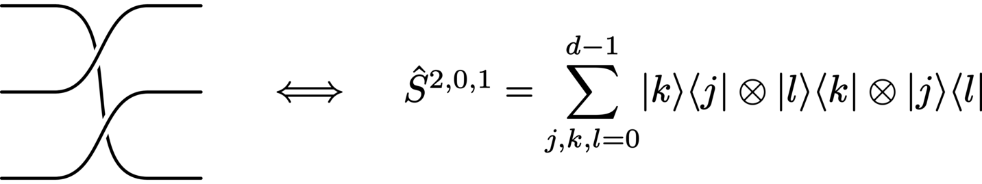
SWAP (exchange):


PSWAP (power-SWAP):


PERM (permutation):
HAD (Hadamard):


QFT (quantum Fourier transform):


CNOT (controlled-NOT):


CCNOT (controlled-controlled-NOT gate, doubly-controlled-NOT gate, also known as the Toffoli gate):


CSUM (controlled-SUM):


CSWAP (controlled-SWAP, also known as the Fredkin gate):


Examples#
A better understanding of quantum circuitry notation can be gained by studying a few basic examples. Perhaps the simplest complete quantum circuit that we can construct consists of just a unipartite quantum state \(\StateDensity\) which evolves into the future along a single quantum wire, subsequently becoming the output state \(\StateDensity^\prime\):


As there are no operations (such as gates or measurements) on the wire, the explicitly labelled output state \(\StateDensity^\prime\) is identically equal to the input state \(\StateDensity\) (since the quantum wire directly connects the two).
If we were to place a gate corresponding to an arbitrary unitary operator \(\Unitary\) upon the intermediary wire, the action from the resulting operation is the standard transformation of a matrix by a linear operator:


In the case of a pure (vector) input state, the circuit is simply:


In this case, we could, without loss of generality, denote the output state with a vector state (such as \(\ket{\StateVector^\prime} = \Unitary\ket{\StateVector}\), equivalent to \(\StateDensity^\prime = \ket{\StateVector^\prime}\bra{\StateVector^\prime}\)), since the action of the (linear transformation) unitary gate preserves the purity of the systems on which it acts. Note that this is not true in general for all circuits; (non-unitary) operations like the (partial) trace do not necessarily preserve the purity of a particular system, and so the output states cannot always be denoted by vector states even if the input states are pure.
More interesting cases are those of multipartite systems. For instance, the evolution of a bipartite input state under a composite unitary gate is:


The evolution of the same state under parallel operations appears as:


In the case where the input state is explicitly separable, we write:


Due to the input state’s separability, the mathematics corresponding to parallel operations on these systems may be greatly simplified:


This is, of course, simply equivalent to two distinct subcircuits with the outputs \(\StateDensity^\prime_A = \Unitary_A \StateDensity_A \Unitary_A^\dagger\) and \(\StateDensity^\prime_B = \Unitary_B \StateDensity_B \Unitary_B^\dagger\), respectively.
Note
For more examples, see the Examples section.
Remarks#
Matrix vs. vector circuits#
Note that our description of quantum circuits thus far has considered quantum processes involving both matrix states (such as mixed states and matrix representations of pure states) and vector states. Traditionally however, quantum circuit diagrams were used exclusively to visualize completely vector processes: all inputs are vector states, all intermediate operations are linear transformations, and so accordingly all outputs are vectors (up until any non-linear operations such as measurement). In such a paradigm, the mathematics corresponding to any given quantum circuit is necessarily always expressible as (linear and unitary) operations on vectors. It is therefore not necessary to express the circuit output using density matrices (such as outer products like \(\ket{\StateVector^\prime}\bra{\StateVector^\prime}\)) in the case of exclusively purity-preserving operations. For example, we may write


which is purely a vector description. In our combined matrix and vector formalism, we can equivalently express the above circuit as


where, despite the vector input and linear transformation, the output is given as a (density) matrix. The circuit formalism presented here is thus a more general one, such that the quantum circuits describe operations on (density) matrix states, not just vector states. This additionally means that both purity-preserving and purity-non-preserving operations (such as the partial trace) are completely captured by our methodology. Note however that in cases where a pure state output is obtained, it is often useful to specify such output in vector form (this being the most compact way of expressing pure states).
References
M. Nielsen and I. Chuang, Quantum Computation and Quantum Information: 10th Anniversary Edition, Cambridge University Press, Cambridge, 2010.
M. M. Wilde, Quantum Information Theory, Cambridge University Press, Cambridge, 2nd edition, 2017.
C. P. Williams, Explorations in Quantum Computing, Springer, London, 2nd edition, December 2010.
V. Moret-Bonillo, Adventures in Computer Science: From Classical Bits to Quantum Bits, Springer International Publishing, Cham, 2017.
M. A. Serrano, R. Pérez-Castillo, and M. Piattini (editors), Quantum Software Engineering, Springer International Publishing, Cham, 2022.
R. P. Feynman, “Quantum mechanical computers”, Foundations of Physics, 16(6):507–531, June 1986. https://doi.org/10.1007/BF01886518, doi:10.1007/BF01886518
A. Kay, “Tutorial on the Quantikz Package”, 2019. http://arxiv.org/abs/1809.03842, doi:10.17637/rh.7000520