Quantum mechanics on discrete Hilbert spaces

The theory of quantum mechanics seeks to explain the dynamics of the particles of which our universe is composed. It differs from classical physics in that certain properties (such as energy and momentum) of bound systems are restricted to being within sets of discrete values—a characteristic known as quantization. Additionally, objects described by quantum mechanics have properties distinctive of both waves and particles (termed wave-particle duality), and there are fundamental limits to the accuracy with which values of specific physical quantities can be predicted prior to their measurement (described by the uncertainty principle). The theory presented here is based on the treatments in [1, 5, 7, 9, 10, 2, 4, 12, 6, 8, 11].

Quantum states

In a formal setup, any system in the discrete theory of quantum mechanics is a collection of identifiable physical properties at a given time. This is represented by a Hilbert space, which may be either infinite- or finite-dimensional. A usual presentation of that Hilbert space is a special function space, such as \(\ell^2\) or \(\Complexes^\Dimension\).

A quantum state is then simply a particular value (or, more properly, a probabilistic assignment) of these properties. It is this object which provides the probability distribution for the outcomes of each possible measurement on a system. Formally, we say that a quantum state represents (or is characterized by) a statistical ensemble \(\SetProbability = \{p_i\}_i\) of independent, identically prepared copies of a quantum system. This is represented in general by a positive semi-definite Hermitian operator \(\StateDensity\) of trace one (that is, a density operator) on the (discrete) Hilbert space \(\SpaceHilbert\). As the space of all density operators on \(\SpaceHilbert\) is convex, then subsequently any convex combination of such operators is also a density operator, which allows us to express any \(\StateDensity\) as

(115)\[\StateDensity = \sum_{i} p_i \StateDensity_i.\]

This describes a mixture of the density operators \(\{\StateDensity_i\}_i\) corresponding to the statistical ensemble \(\SetProbability\). According to the spectral theorem (63), we are able to express any quantum state \(\StateDensity\) in a \(\Dimension\)-dimensional Hilbert space \(\SpaceHilbert\) equivalently as a convex combination of at most \(\Dimension\) vectors \(\{\ket{\psi_i}\}_i\), i.e.,

(116)\[\StateDensity = \sum_{i} p_i \ket{\psi_i}\bra{\psi_i}\]

where the coefficients \(\{p_i\}_i\) collectively characterize \(\StateDensity\).

Pure states

An extreme point in the convex space spanned by operators (115) is called a pure state, which we can denote in general as the outer product

(117)\[\StateDensity = \ket{\psi}\bra{\psi}.\]

This is necessarily a projection operator, i.e., \(\StateDensity^2 = \StateDensity\). Due to this form, any given pure state can be completely (and uniquely) represented by the vector

(118)\[\ket{\psi} = \sum_{i} c_i \ket{\Basis_i}\]

where \(\{\ket{\Basis_i}\}_i\) is an orthonormal basis for the associated Hilbert space, and \(c_i \in \Complexes\) are the state-characterizing probability amplitudes.

The set of physical pure states \(\SpacePure(\SpaceHilbert)\) on a Hilbert space \(\SpaceHilbert\) is the set of all normalized (unit) vectors on \(\SpaceHilbert\), with vectors equal up to a global phase considered to be equivalent (as such global phase differences are not observable, i.e., constitute measurable quantities). Compactly, we write

(119)\[\SpacePure(\SpaceHilbert) \equiv \bigl\{ \ket{\psi} \in \SpaceHilbert : \norm{\ket{\psi}}_2 = 1, \, \ket{\psi} \cong \e^{\eye \theta} \ket{\psi} \, \, \forall \, \, \theta \in \Reals \bigr\}.\]

Note

The concept of vectors which differ only up to a multiplicate constant of magnitude \(1\) (i.e., a phase factor \(\e^{\eye \theta}\)) being identified is a direct consequence of the fact that such states are physically indistinguishable—that is, there is no performable experiment which is able to differentiate them. This leads to the idea that the notion of a pure “state” in quantum mechanics is perhaps better described by a more complete (and unique) object called a ray, residing in a projective Hilbert space. Put simply, a ray \(\underline{\StatePure}\) is the set of all state vectors \(\StatePure\) which are scalar non-zero multiples of each other, i.e.,

(120)\[\underline{\StatePure} = \bigl\{\e^{\eye \theta} \StatePure : \StatePure \in \SpaceHilbert, \, \norm{\psi}_2 = 1, \, \theta \in \Reals \bigr\}.\]

The vectors in this set are all physically equivalent and called representants of \(\underline{\StatePure}\). For example, if \(\psi \in \underline{\psi}\), then \(\phi\) is also a representant of \(\underline{\psi}\) if and only if \(\phi = \e^{\eye \theta}\psi\) for some \(\theta \in \Reals\), and therefore corresponds to the same physical state. In fact, in this formalism, a (pure) “quantum state” is more properly identified as the ray itself, not just a (single) vector. Given a Hilbert space \(\SpaceHilbert\), any two \(\psi_1,\psi_2 \in \SpaceHilbert\) satisfy the equivalence relation \(\psi_1 \sim \psi_2\) if and only if \(\psi_1,\psi_2 \in \underline{\psi}\). As such, the rays of \(\SpaceHilbert\) form the equivalence classes of this equivalence equation, which correspond physically to distinguishable quantum states. Thus, when we (imprecisely) describe a quantum state using a vector \(\ket{\StatePure}\) in the context of quantum mechanics, we systematically use any one element of the corresponding ray as its representant, albeit with the specific choice being completely inconsequential to any predictions of the theory.

Mixed states

States which are not pure are termed mixed, and cannot be expressed in the form (117). A mixed state characterized by a uniform probability distribution \(\SetProbability\) is called maximally mixed and takes the form

(121)\[\StateDensity = \frac{1}{\Dimension}\Identity_{\Dimension}\]

where \(\Identity_{\Dimension}\) is the \(\Dimension \times \Dimension\) identity operator. It is useful to think of linear combinations such as that in (116) as “classical” superpositions in the sense that they involve the correspondingly classical mixing of otherwise fully quantum-mechanical states \(\StateDensity_i = \ket{\psi_i}\bra{\psi_i}\). In other words, a mixed quantum state is a statistical ensemble of pure states, and is also known simply as a mixed ensemble. Importantly, this contrasts with the physically distinct notion of quantum superposition, which is encapsulated by (118).

Unlike pure states, mixed states cannot be represented as a state vector (e.g., \(\ket{\psi}\)). Both objects however may be described as a density operator (e.g., \(\StateDensity\)), which serves as a generalization of the concept of state vectors (wave functions). The set of physical density operators (including both pure and mixed states) on a Hilbert space \(\SpaceHilbert\) is the set of all Hermitian trace-one (linear) operators on \(\SpaceHilbert\), and we denote this as

(122)\[\SpaceMixed(\SpaceHilbert) \equiv \bigl\{ \StateDensity \in \SpaceLinear(\SpaceHilbert) : \StateDensity^\dagger = \StateDensity, \, \trace[\StateDensity] = 1 \bigr\}.\]

Density operators representing mixed (impure) quantum states arise in quantum mechanics in two distinct situations. The first of these is when the preparation of a system is not fully known. In this case, the (incomplete/limited) knowledge of the quantum state can be captured only by a density operator that describes a statistical (i.e., mixture) of all possible preparations. The second situation is when one wants to describe a physical system that is entangled with another. Quantum entanglement theoretically prevents the existence of complete knowledge about subsystems in an entangled state, and so it is impossible to represent the state of any such subsystems as a pure state.

Note

A useful concept in the formalism of quantum information theory is that of purification. This process refers to the fact that any mixed state in a finite-dimensional Hilbert space can be viewed as the reduced state of some pure state. To see this, let \(\StateDensity \in \SpaceMixed(\SpaceHilbert_A)\) be a density matrix where \(\dim(\SpaceHilbert_A)\) is finite. Given this, it is always possible to introduce an additional Hilbert space \(\SpaceHilbert_B\), corresponding to a fictitious system often called a reference system (and has no direct physical significance), alongside a pure state \(\ket{\psi} \in \SpacePure(\SpaceHilbert_A \otimes \SpaceHilbert_B)\) such that

(123)\[\trace_B \bigl[\ket{\psi}\bra{\psi}\bigr] = \StateDensity.\]

We say that \(\ket{\psi}\) purifies \(\StateDensity\), which is a consequence that is only made possible by the fact that we have access to a larger (composite) Hilbert space.

Qubits

Many physical applications of this theory in quantum mechanics involve Boolean (i.e., binary, or two-valued) logic, which is completely describable by exactly two orthonormal vectors that are often labelled \(\ket{0}\) and \(\ket{1}\). The representations in \(\Complexes^2\) of these vectors is typically the pair

(124)\[\begin{split}\ket{0} = \begin{bmatrix} 1 \\ 0 \end{bmatrix}, \qquad \ket{1} = \begin{bmatrix} 0 \\ 1 \end{bmatrix}.\end{split}\]

Together, these form a complete basis that is canonically known as the \(z\)-basis (given that each vector is an eigenvector of the Pauli-\(Z\) operator \(\Pauli_z\) (130)), though is alternatively often referred to by many simply as the computational basis. Any quantum state with such binary dimensionality is called a qubit (though this nomenclature is often used solely in the context of pure binary states), and describes a two-level system that forms the basic unit of quantum information (analogous to the bit in classical computing). In the computational basis \(\{\ket{0},\ket{1}\}\), the simplest qubit which we can express is the quantum superposition

(125)\[\ket{\StateVector} = \alpha\ket{0} + \beta\ket{1}, \quad \abs{\alpha}^2 + \abs{\beta}^2 = 1, \quad \alpha,\beta \in \Complexes.\]

In the \(\Complexes^2\)-representation (124), this state can be expressed as

(126)\[\begin{split}\ket{\StateVector} = \alpha \begin{bmatrix} 1 \\ 0 \end{bmatrix} + \beta \begin{bmatrix} 0 \\ 1 \end{bmatrix} = \begin{bmatrix} \alpha \\ \beta \end{bmatrix}.\end{split}\]

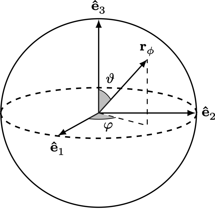
An alternative parametrisation of the qubit vector state (125) takes the form

(127)\[\ket{\StateVector} = \e^{\eye\varsigma}\left[\cos\biggl(\frac{\vartheta}{2}\biggr)\ket{0} + \e^{\eye\varphi}\sin\biggl(\frac{\vartheta}{2}\biggr)\ket{1}\right], \quad \varsigma,\vartheta,\varphi \in \Reals.\]

Given that the factor \(\e^{\eye\varsigma}\) represents a global phase, then all states with fixed \(\vartheta,\varphi\) but different \(\varsigma\) are physically equivalent, and so this factor can be disregarded. We are therefore left with a parametrization of a qubit wherein the numbers \(\vartheta\) and \(\varphi\) define a point on the surface of a unit sphere, known as the Bloch sphere (illustrated in Figure 1). This is essentially a unique mapping of the \(2\)-dimensional Hilbert space to the \(3\)-dimensional real space \(\Reals^3\) (with basis vectors \(\{\uv{e}_1,\uv{e}_2,\uv{e}_3\}\)), which is accomplished by choosing the antipodal points on unit sphere in \(\Reals^3\) to correspond to the pair of mutually orthogonal basis vectors \(\ket{0}\) and \(\ket{1}\). In this sense, the qubit state \(\vec{r}_\StateVector \in \Reals^3\), which corresponds to its Hilbert space counterpart (125), may be written exactly as

(128)\[\vec{r}_\StateVector = \sin(\vartheta)\cos(\varphi)\uv{e}_1 + \sin(\vartheta)\sin(\varphi)\uv{e}_2 + \cos(\vartheta)\uv{e}_3.\]

Similarly, a \(2\)-dimensional density operator \(\StateDensity\) in the same representation corresponds to the vector

(129)\[\vec{r}_{\StateDensity} = \trace[\StateDensity \Pauli_1]\uv{e}_1 + \trace[\StateDensity \Pauli_2]\uv{e}_2 + \trace[\StateDensity \Pauli_3]\uv{e}_3\]

where

(130)\[\begin{split}\begin{aligned} \Pauli_1 &= \Pauli_x \equiv \ket{0}\bra{1} + \ket{1}\bra{0} \!\!\!\!\!\! & &= \begin{bmatrix} 0 & 1 \\ 1 & 0 \end{bmatrix}, \\ \Pauli_2 &= \Pauli_y \equiv -\eye \ket{0}\bra{1} + \eye \ket{1}\bra{0} \!\!\!\!\!\! & &= \begin{bmatrix} 0 & -\eye \\ \eye & 0 \end{bmatrix}, \\ \Pauli_3 &= \Pauli_z \equiv \ket{0}\bra{0} - \ket{1}\bra{1} \!\!\!\!\!\! & &= \begin{bmatrix} 1 & 0 \\ 0 & -1 \end{bmatrix}, \end{aligned}\end{split}\]

are the Pauli matrices.

Figure 1 The Bloch sphere.

The Pauli matrices \(\{\Pauli_k\}_{k=1}^{3}\) are Hermitian, and so represent observables in the context of quantum mechanics. Together with the identity operator (writing \(\Pauli_0 = \Identity_2\)), the set \(\{\Pauli_\mu\}_{\mu=0}^{3}\) forms a complete basis for the space of complex \(2 \times 2\) matrices. Since this coincides with the space of linear operators \(\SpaceLinear(\SpaceHilbert)\) on a qubit Hilbert space \(\SpaceHilbert\), then any (density) operator \(\StateDensity \in \SpaceLinear(\SpaceHilbert)\) can be expressed as the linear combination

(131)\[\StateDensity = \frac{1}{2}\sum_{\mu=0}^{3} \trace[\Pauli_\mu \StateDensity]\Pauli_\mu.\]

In the context of density operators, since the coefficient for \(\mu = 0\) in (131) is fixed by normalization (i.e., \(\trace[\Pauli_0 \StateDensity] = 1\)), then the state \(\StateDensity\) is completely (and uniquely) determined by the Bloch vector, which is defined for a \(\Dimension\)-dimensional state as the \((\Dimension^2 - 1)\)-dimensional real vector of parameters \(\bigl\{\trace[\Pauli_k \StateDensity]\bigr\}_{k = 1}^{\Dimension^2 - 1}\). Accordingly, the linear combination (131) is said to be the Bloch sphere representation of the state \(\StateDensity\). Note also of course that any appropriate basis, not just the Pauli basis (with identity), allows for reconstruction of any qubit state in the manner of (131).

The Bloch vector provides a complete description of a quantum system because it represents the expectation values of specific informationally complete observables. In general, a complex \(\Dimension \times \Dimension\) density matrix, which represents the state of an \(\Dimension\)-dimensional quantum system, is geometrically equivalent to a vector in an \((\Dimension^2 - 1)\)-dimensional real space. This is because the space of density matrices is a (bounded) convex subset of \(\Reals^{\Dimension^2}\), with its elements possessing certain properties (namely Hermiticity, positive semi-definiteness, and trace equal to \(1\)). Since this real space coincides with that of the (generalized) Bloch ball, including both the surface (the Bloch sphere, on which points correspond to pure states) and interior (in which points correspond to mixed states), then this is why determination of the Bloch vector is equivalent to identification of the quantum state. Therefore, as the Pauli operators form a set of informationally complete observables for qubit systems, then the inclusion of the identity operator to this set yields a tomographically complete basis for the space of \(2 \times 2\) Hermitian matrices, of which the space of \(2\)-dimensional density matrices is a subset.

Qutrits

Quantum states realized by \(3\)-dimensional systems are commonly known as qutrits. These objects are analogous to the “trit” unit of information in classical computing and so are useful for performing calculations with ternary logic. Such systems are typically described using a set of orthonormal (basis) vectors \(3\)-dimensional \(\{\ket{0},\ket{1},\ket{2}\}\), with which a qutrit can in general be expressed as

(132)\[\ket{\StateVector} = \alpha\ket{0} + \beta\ket{1} + \gamma\ket{2}, \quad \abs{\alpha}^2 + \abs{\beta}^2 + \abs{\gamma}^2 = 1, \quad \alpha,\beta,\gamma \in \Complexes.\]

In the \(\Complexes^3\)-representation, the basis vectors often take the forms

(133)\[\begin{split}\ket{0} = \begin{bmatrix} 1 \\ 0 \\ 0 \end{bmatrix}, \qquad \ket{1} = \begin{bmatrix} 0 \\ 1 \\ 0 \end{bmatrix}, \qquad \ket{2} = \begin{bmatrix} 0 \\ 0 \\ 1 \end{bmatrix},\end{split}\]

with which (132) can be rewritten as

(134)\[\begin{split}\ket{\StateVector} = \alpha \begin{bmatrix} 1 \\ 0 \\ 0 \end{bmatrix} + \beta \begin{bmatrix} 0 \\ 1 \\ 0 \end{bmatrix} + \gamma \begin{bmatrix} 0 \\ 0 \\ 1 \end{bmatrix} = \begin{bmatrix} \alpha \\ \beta \\ \gamma \end{bmatrix}.\end{split}\]

Qutrits described by \(3\)-dimensional density operators have corresponding representations as \(3 \times 3\) density matrices. One way of expressing such a state is via the linear combination

(135)\[\StateDensity = \frac{1}{3}\sum_{\mu=0}^{8} \trace[\GellMann_\mu \StateDensity]\GellMann_\mu.\]

where \(\{\Pauli_\mu\}_{\mu=0}^{3}\) is a complete basis for the space of \(3 \times 3\) complex matrices. Perhaps the most notable choice of matrices with which to construct a such a basis are the Gell-Mann matrices,

(136)\[\begin{split}\begin{aligned} \GellMann_1 &\equiv \ket{0}\bra{1} + \ket{1}\bra{0} \!\!\!\!\!\! & &= \begin{bmatrix} 0 & 1 & 0 \\ 1 & 0 & 0 \\ 0 & 0 & 0 \end{bmatrix}, \\ \GellMann_2 &\equiv -\eye\ket{0}\bra{1} + \eye \ket{1}\bra{0} \!\!\!\!\!\! & &= \begin{bmatrix} 0 & -\eye & 0 \\ \eye & 0 & 0 \\ 0 & 0 & 0 \end{bmatrix}, \\ \GellMann_3 &\equiv \ket{0}\bra{0} - \ket{1}\bra{1} \!\!\!\!\!\! & &= \begin{bmatrix} 1 & 0 & 0 \\ 0 & -1 & 0 \\ 0 & 0 & 0 \end{bmatrix}, \\ \GellMann_4 &\equiv \ket{0}\bra{2} + \ket{2}\bra{0} \!\!\!\!\!\! & &= \begin{bmatrix} 0 & 0 & 1 \\ 0 & 0 & 0 \\ 1 & 0 & 0 \end{bmatrix}, \\ \GellMann_5 &\equiv -\eye\ket{0}\bra{2} + \eye\ket{2}\bra{0} \!\!\!\!\!\! & &= \begin{bmatrix} 0 & 0 & -\eye \\ 0 & 0 & 0 \\ \eye & 0 & 0 \end{bmatrix}, \\ \GellMann_6 &\equiv \ket{2}\bra{3} + \ket{3}\bra{2} \!\!\!\!\!\! & &= \begin{bmatrix} 0 & 0 & 0 \\ 0 & 0 & 1 \\ 0 & 1 & 0 \end{bmatrix}, \\ \GellMann_7 &\equiv -\eye\ket{2}\bra{3} + \eye\ket{3}\bra{2} \!\!\!\!\!\! & &= \begin{bmatrix} 0 & 0 & 0 \\ 0 & 0 & -\eye \\ 0 & \eye & 0 \end{bmatrix}, \\ \GellMann_8 &\equiv \frac{1}{\sqrt{3}}\bigl(\ket{0}\bra{0} + \ket{1}\bra{1} - 2\ket{2}\bra{2}\bigr) \!\!\!\!\!\! & &= \frac{1}{\sqrt{3}}\begin{bmatrix} 1 & 0 & 0 \\ 0 & 1 & 0 \\ 0 & 0 & -2 \end{bmatrix}, \end{aligned}\end{split}\]

in addition to \(\GellMann_0 \equiv \Identity_3\).

Qudits

Quantum vector states in a \(\Dimension\)-dimensional Hilbert space \(\SpaceHilbert_\Dimension\) can in general be expressed as the superposition

(137)\[\ket{\StateVector} = \sum_{i=0}^{\Dimension - 1} c_i \ket{i}, \quad \sum_{i=0}^{\Dimension - 1} \abs{c_i}^2 = 1, \quad c_i \in \Complexes.\]

which is often referred to as a qudit. Here, \(\{\ket{i}\}_{i=0}^{\Dimension - 1}\) is a vector basis for \(\SpaceHilbert_\Dimension\), and may be expressed in a \(\Complexes^\Dimension\)-representation using the vectors in (37). With this, we can write (137) as

(138)\[\begin{split}\ket{\StateVector} = c_0 \begin{bmatrix} 1 \\ 0 \\ \vdots \\ 0 \end{bmatrix} + c_1 \begin{bmatrix} 0 \\ 1 \\ \vdots \\ 0 \end{bmatrix} + \ldots + c_{\Dimension - 1} \begin{bmatrix} 0 \\ 0 \\ \vdots \\ 1 \end{bmatrix} = \begin{bmatrix} c_0 \\ c_1 \\ \vdots \\ c_{\Dimension - 1} \end{bmatrix}.\end{split}\]

Just like in the cases of qubits and qutrits, general \(\Dimension\)-dimensional states described by density operators can be expressed via a linear combination of the form

(139)\[\StateDensity = \frac{1}{\Dimension}\sum_{\mu=0}^{\Dimension^2 - 1} \trace[\GellMann_\mu \StateDensity]\GellMann_\mu.\]

In order for this to be true, the matrices \(\{\GellMann_\mu\}_{\mu=0}^{\Dimension^2 - 1}\) must form a basis for the space of \(\Dimension \times \Dimension\) density matrices. Though there are multiple ways to find such a basis, doing so is a non-trivial task. Our construction here closely follows the work of [2], in which a suitable generalization of the Gell-Mann (or Pauli) matrices (136) is obtained. We begin by introducing the elementary matrices \(\{\Basis_{i}^{j}\}_{i,j = 1}^{\Dimension}\) which satisfy

(140)\[(\Basis_{i}^{j})_{nm} = \delta_{ni} \delta_{mj}, \qquad 1 \leq n \leq d, \quad 1 \leq m \leq d.\]

This defines a total of \(\Dimension^2\) matrices, each of which possesses one entry equal to unity and all others equal to zero. Using these, we can construct \(\Dimension (\Dimension - 1)\) traceless off-diagonal matrices,

(141)\[\begin{split}\begin{aligned} \alpha_{i}^{j} &= \Basis_{i}^{j} + \Basis_{j}^{i} \\ \beta_{i}^{j} &= -\eye(\Basis_{i}^{j} - \Basis_{j}^{i}), \qquad 1 \leq j < i \leq d \end{aligned}\end{split}\]

and \(\Dimension - 1\) traceless diagonal matrices,

(142)\[\gamma_{j}^{j} = \sqrt{\frac{2}{j(j+1)}} \left[\sum_{k=1}^{j} \Basis_{k}^{k} - j \Basis_{j+1}^{j+1}\right].\]

In total, we obtain \(\Dimension^2 - 1\) traceless matrices. Note that these matrices are in fact the generators of \(\mathrm{SU}(\Dimension)\) (the group of \(\Dimension \times \Dimension\) unitary matrices with determinant \(1\)), meaning that they form a basis for the corresponding Lie algebra \(\mathfrak{su}(\Dimension)\) (the space of \(\Dimension \times \Dimension\) traceless Hermitian matrices). As the space of \(\Dimension \times \Dimension\) Hermitian matrices has a real dimensionality of \(\Dimension^2\), then the difference between this space and \(\mathfrak{su}(\Dimension)\) is a single degree of freedom that accounts for the ability of the matrices in the former to be non-traceless. This missing property can be incorporated into the latter by including the \(\Dimension\)-dimensional identity matrix \(\Identity_\Dimension\) into any of its valid bases. In other words, the set of matrices that consists of both the generators of \(\mathrm{SU}(\Dimension)\) and the identity \(\Identity_\Dimension\) necessarily forms a basis for the entire space of \(\Dimension \times \Dimension\) Hermitian matrices (both traceless and non-traceless).

With this in mind, we can use (141) and (142) to assemble a set of matrices,

(143)\[\begin{split}\begin{aligned} \GellMann_{(i-1)^2 + 2(j - 1)} &\equiv \alpha_{i}^{j}, \\ \GellMann_{(i-1)^2 + 2j - 1} &\equiv \beta_{i}^{j}, \\ \GellMann_{i^2 - 1} &\equiv \gamma_{i-1}^{i-1}. \end{aligned}\end{split}\]

These matrices are known as the generalized Gell-Mann matrices. In conjunction with the identity matrix \(\GellMann_0 \equiv \Identity_\Dimension\), they form a suitable basis for the space of \(\Dimension\)-dimensional Hermitian matrices, meaning that any density matrix can indeed be expressed as the linear combination (139) using this basis.

Quantum quantities

Purity

The mixedness of a state may be quantified by the purity function,

(144)\[\Purity(\StateDensity) \equiv \trace[\StateDensity^2],\]

which defines a measure on the degree by which a state deviates from being (completely) pure. The purity of normalized \(\Dimension\)-dimensional states is bounded from above by \(1\) (perfect purity) and below by \(\frac{1}{\Dimension}\) (maximal mixing), e.g.,

(145)\[\frac{1}{\Dimension} \leq \Purity(\StateDensity) \leq 1,\]

and so a state \(\StateDensity\) is pure if and only if \(\Purity(\StateDensity) = 1\) (else it has some degree of mixing).

Trace distance

The trace distance is a metric on the space of density matrices, thereby providing a measure of the “distance” (or distinguishability) between two states. It is a generalization of the Kolmogorov distance for classical probability distributions to quantum density operators, and is defined for any two such operators \(\op{\rho}\) and \(\op{\tau}\) as

(146)\[\TraceDistance(\op{\rho},\op{\tau}) \equiv \frac{1}{2} \trace | \op{\rho} - \op{\tau} |.\]

Here, we defined \(| \op{A} | \equiv \sqrt{\op{A}^\dagger\op{A}}\) to be the absolute value of an operator \(\op{A}\). Being a metric, the trace distance between density operators is always non-negative, i.e.,

(147)\[\TraceDistance(\op{\rho},\op{\tau}) \geq 0,\]

with equality (with zero) if and only if \(\op{\rho} = \op{\tau}\). It is also necessarily symmetric, e.g., \(\TraceDistance(\op{\rho},\op{\tau}) = \TraceDistance(\op{\tau},\op{\rho})\), and satisfies the triangle inequality, e.g.,

(148)\[\TraceDistance(\op{\rho},\op{\tau}) \leq \TraceDistance(\op{\rho},\op{\sigma}) + \TraceDistance(\op{\sigma},\op{\tau}),\]

for all density operators \(\op{\rho}\), \(\op{\tau}\), and \(\op{\sigma}\). In the case of normalized quantum states, the trace distance is bounded from above by unity, e.g.,

(149)\[0 \leq \TraceDistance(\op{\rho},\op{\tau}) \leq 1.\]

Fidelity

Another measure between two quantum states is the fidelity, which characterizes their similarity or “closeness”. It is defined for two density operators \(\op{\rho}\) and \(\op{\tau}\) as

(150)\[\Fidelity(\op{\rho},\op{\tau}) \equiv \left(\trace\sqrt{\sqrt{\op{\rho}} \, \op{\tau}\sqrt{\op{\rho}}}\right)^2,\]

where the square roots of \(\op{\rho}\) and \(\sqrt{\op{\rho}} \, \op{\tau}\sqrt{\op{\rho}}\) (both positive-semidefinite matrices) are well-defined by the spectral theorem (63). While the fidelity is not a suitable metric on the space of density matrices, it still provides many of the properties that are expected of a useful distance measure. For example, it is non-negative for any input, e.g.,

(151)\[0 \leq \Fidelity(\op{\rho},\op{\tau}) \leq 1,\]

with equivalence to its upper bound of unity if and only if \(\op{\rho} = \op{\tau}\).

The fidelity expressed in (150) is the original, traditional form that is often cumbersome to use and inefficient to compute. Simpler yet equivalent reformulations are therefore desired, with perhaps the most encountered of such expressions being

(152)\[\Fidelity(\op{\rho},\op{\tau}) \equiv \left(\trace\bigl|\sqrt{\op{\rho}} \sqrt{\op{\tau}}\bigr|\right)^2,\]

where \(| \op{A} | \equiv \sqrt{\op{A}^\dagger\op{A}}\). Recent work [13, 14] has shown that, by leveraging the fact that the trace of a diagonalizable square matrix is equal to the sum of its eigenvalues, an even simpler expression for the fidelity can be written as

(153)\[\Fidelity(\op{\rho},\op{\tau}) \equiv \left(\trace\sqrt{\op{\rho} \op{\tau}}\right)^2,\]

which holds true regardless of whether \(\op{\rho}\) and \(\op{\tau}\) do or do not commute.

In the case where either density matrix is pure, we can write

(154)\[\begin{split}\Fidelity(\op{\rho},\op{\tau}) = \trace[\op{\rho}\op{\tau}] = \begin{cases} \langle \psi_\rho | \op{\tau} | \psi_\rho \rangle, & \text{if } \op{\rho} = | \psi_\rho \rangle \langle \psi_\rho |; \\ \langle \psi_\tau | \op{\rho} | \psi_\tau \rangle, & \text{if } \op{\tau} = | \psi_\tau \rangle \langle \psi_\tau |; \\ \end{cases}\end{split}\]

which further reduces to the overlap

(155)\[\Fidelity(\op{\rho},\op{\tau}) = \abs{\langle \psi_\rho | \psi_\tau \rangle}^2\]

when both states are pure.

Lastly, note that an alternative definition of the fidelity exists that specifies the same expression as (150) except without the square, i.e.,

(156)\[\Fidelity(\op{\rho},\op{\tau}) \equiv \trace\sqrt{\sqrt{\op{\rho}} \, \op{\tau}\sqrt{\op{\rho}}}.\]

This form, sometimes called the root fidelity, shares many of the same properties as (150), but is ostensibly less common in the literature.

Entropy

In statistical physics, the concept of entropy commonly provides a quantification of how much uncertainty there is in the state of a physical system. In other words, it characterizes the “amount” of mixedness of a quantum state (that is, the degree to which the state is mixed). For quantum systems, the standard measure of entropy is the von Neumann entropy, defined for an arbitrary state \(\StateDensity\) as

(157)\[\Entropy(\StateDensity) \equiv -\trace[\StateDensity \log_\Base \StateDensity].\]

This definition can be equivalently expressed as

(158)\[\Entropy(\StateDensity) = -\sum_{k} \lambda_k \log_\Base \lambda_k\]

where \(\lambda_k\) denote the non-zero eigenvalues in the spectrum of \(\StateDensity\). Here, the matrix logarithm is taken to base \(\Base\), which is the dimensionality of the unit of information in which the entropy is measured. For example, if \(\Base = 2\), then \(\Entropy(\StateDensity)\) will be measured in “bits”. Many definitions of the von Neumann entropy alternatively specify \(\Base = \e\), for which the entropy is measured in so-called “nats”.

The von Neumann entropy is the quantum counterpart of the Shannon entropy in classical information theory. For a pure state, it is always zero, while for a mixed state, it is strictly positive with an upper bound of \(\log_\Base \Dimension\) (achieved with a maximally mixed state) in a unipartite \(\Dimension\)-dimensional Hilbert space. Mathematically, we can write

(159)\[0 \leq \Entropy(\StateDensity) \leq \log_\Base \Dimension\]

with \(\Entropy(\StateDensity) = 0\) if and only if \(\StateDensity\) is pure.

The quantum relative entropy provides a measure of distinguishability between two quantum density matrices, and is defined as

(160)\[\begin{split}\begin{aligned} \Entropy(\op{\rho} \Vert \op{\tau}) &\equiv -\trace[\op{\rho} \log_\Base \op{\tau}] - \Entropy(\op{\rho}) \\ &= \trace\bigl[\op{\rho}(\log_\Base \op{\rho} - \log_\Base \op{\tau})\bigr], \end{aligned}\end{split}\]

where \(\op{\rho}\) and \(\op{\tau}\) are arbitrary quantum states of the same dimensionality. It is analogous to the notion of relative entropy from classical information theory, wherein it characterizes the “distance” between two probability distributions. Klein’s inequality states that the quantum relative entropy is non-negative, i.e.,

(161)\[\Entropy(\op{\rho} \Vert \op{\tau}) \geq 0,\]

for any two density matrices \(\op{\rho}\) and \(\op{\tau}\), with equality if and only if \(\op{\rho} = \op{\tau}\).

Mutual information

The quantum mutual information is a measure of correlation between the subsystems of a multipartite quantum system. Let \(\op{\rho}^{A,B}\) be a bipartite state for a composite system with Hilbert space \(\SpaceHilbert_A \otimes \SpaceHilbert_B\), and let

(162)\[\begin{split}\begin{aligned} \op{\rho}^{A} &\equiv \trace_B[\op{\rho}^{A,B}], \\ \op{\rho}^{B} &\equiv \trace_A[\op{\rho}^{A,B}], \end{aligned}\end{split}\]

be the reduced states on subsystems \(A\) and \(B\), respectively. Using these, we can define the mutual information between these subsystems as

(163)\[\MutualInformation(A : B) \equiv \Entropy(\op{\rho}^{A}) + \Entropy(\op{\rho}^{B}) - \Entropy(\op{\rho}^{A,B}),\]

where \(\Entropy(\op{\rho})\) is the von Neumann entropy of a state \(\op{\rho}\) as defined in (157). An equivalent expression uses the relative entropy (160) to write

(164)\[\MutualInformation(A : B) = \Entropy(\op{\rho}^{A,B} \Vert \op{\rho}^{A} \otimes \op{\rho}^{B}).\]

The quantum mutual information is analogous to the Shannon mutual information in classical information theory. It is a non-negative quantity, i.e.,

(165)\[\MutualInformation(A : B) \geq 0,\]

with equality if and only if the subsystems are independent (and are thus uncorrelated).

Separability and entanglement

A vector state \(\ket{\psi} \in \SpacePure(\SpaceHilbert_0 \otimes \SpaceHilbert_1 \otimes \ldots \otimes \SpaceHilbert_{N - 1})\) over \(N\) subsystems is called separable or a product state if it can be written in the form

(166)\[\begin{split}\begin{aligned} \ket{\psi} &= \ket{\psi_0} \otimes \ket{\psi_1} \otimes \ldots \otimes \ket{\psi_{N - 1}} \\ &= \bigotimes_{n=0}^{N - 1} \ket{\psi_n}, \end{aligned}\end{split}\]

where \(\ket{\psi_n} \in \SpacePure(\SpaceHilbert_n)\) is a vector state on the \(n\)-th subsystem. Similarly, a mixed state \(\StateDensity \in \SpaceMixed(\SpaceHilbert_0 \otimes \SpaceHilbert_1 \otimes \ldots \otimes \SpaceHilbert_{N - 1})\) over \(N\) subsystems is separable if it can be expressed as

(167)\[\begin{split}\begin{aligned} \StateDensity &= \sum_{k} p_k \StateDensity_k^0 \otimes \StateDensity_k^1 \otimes \ldots \otimes \StateDensity_k^{N - 1} \\ &= \sum_{k} p_k \bigotimes_{n=0}^{N - 1} \StateDensity_k^n, \end{aligned}\end{split}\]

where \(\StateDensity_k^n \in \SpaceMixed(\SpaceHilbert_n)\) are density operators representing the \(n\)-th subsystem, and the coefficients \(p_k\) are non-negative real numbers that collectively satisfy \(\sum_{k} p_k = 1\). If there exists only a single non-zero \(p_k\), then the state is called simply separable or, similarly to the separable vector state case, a product state.

A quantum state that is not separable (termed non-separable) is said to be entangled. The corresponding phenomenon, quantum entanglement, is one of the most fascinating features of quantum mechanics. It manifests physically as quantum correlations (of various quantum properties such as observable quantities) between the individual subsystems of a composite quantum system. For example, a group of particles is entangled when the quantum state of each individual particle cannot be described independently of the state of the other particles in a collective description. This behaviour is realized to varying degrees in many different kinds of physical situations, including most interestingly when the particles are spacelike separated.

Quantum entanglement is also necessarily characterized by unrealized correlations, such that the outcomes of measurements on the quantum system(s) are completely undecided until the measurement occurs. This means that the very act of performing a measurement on one subsystem of an entangled composition affects the entire system as a whole (i.e., apparent and irreversible collapse of the wave function). Though any such influence occurs seemingly instantaneously, quantum entanglement however does not allow any information to propagate superluminally (i.e., faster than the speed of light), despite the possibility that the subsystems of an entangled system are spacelike separated.

A quantum system is said to be maximally entangled if it cannot be separated into pure states on each of its subsystems. This can only occur between exactly two particles, which is to say that a single particle cannot be maximally entangled with more than one other particle at a time. This is a property called monogamy, and is a restriction that results in perfect quantum correlations between any two such entangled subsystems. For qubits, the maximally entangled states are the Bell states, of which there are four:

(168)\[\begin{split}\begin{aligned} \ket{\Phi^+} &\equiv \frac{1}{\sqrt{2}} \bigl(\ket{0} \otimes \ket{0} + \ket{1} \otimes \ket{1} \bigr), \\ \ket{\Phi^-} &\equiv \frac{1}{\sqrt{2}} \bigl(\ket{0} \otimes \ket{0} - \ket{1} \otimes \ket{1} \bigr), \\ \ket{\Psi^+} &\equiv \frac{1}{\sqrt{2}} \bigl(\ket{0} \otimes \ket{1} + \ket{1} \otimes \ket{0} \bigr), \\ \ket{\Psi^-} &\equiv \frac{1}{\sqrt{2}} \bigl(\ket{0} \otimes \ket{1} - \ket{1} \otimes \ket{0} \bigr). \end{aligned}\end{split}\]

For systems composed of three or more subsystems (e.g., particles), any multipartite entanglement that manifests cannot be maximal as in the bipartite case (due to the monogamy), but still exists in many quantitatively different types. An example of an entangled three-qubit system is the Greenberger-Horne-Zeilinger (GHZ) state,

(169)\[\ket{\mathrm{GHZ}} = \frac{1}{\sqrt{2}} \bigl(\ket{0} \otimes \ket{0} \otimes \ket{0} + \ket{1} \otimes \ket{1} \otimes \ket{1}\bigr).\]

Discarding (tracing out) any of its subsystems results in a separable state. Dissimilarly, for the three-qubit W state,

(170)\[\ket{\mathrm{W}} = \frac{1}{\sqrt{3}} \bigl(\ket{0} \otimes \ket{0} \otimes \ket{1} + \ket{0} \otimes \ket{1} \otimes \ket{0} + \ket{1} \otimes \ket{0} \otimes \ket{0}\bigr),\]

discarding any single subsystem yields a bipartite state that is still entangled.

Quantum operations

A quantum operation is a linear, trace-non-increasing, completely positive map

(171)\[\MapGeneral : \StateDensity \mapsto \MapGeneral[\StateDensity] \in \SpaceMixed(\SpaceHilbert).\]

It is convenient to express such maps using the general form

(172)\[\MapGeneral[\StateDensity] = \sum_{i} \Kraus^\dagger_i \StateDensity \Kraus_i\]

where \(\SetKraus = \{\Kraus_i\}_i\) is a set of linear operators, known as Kraus operators. The characteristic of trace-non-increasing is the requirement that \(\trace[\StateDensity] \geq \trace\bigl[\MapGeneral[\StateDensity]\bigr]\). Since it is (almost) always assumed that the input state \(\StateDensity\) satisfies \(\trace[\StateDensity] = 1\), then the Kraus operators of a trace-non-increasing quantum operation in turn satisfy

(173)\[\sum_{i} \Kraus^\dagger_i \Kraus_i \leq \Identity.\]

In the case of equivalence, the operation is said to be complete (and trace-preserving), otherwise it is incomplete (and trace-decreasing). An operation \(\MapGeneral[\StateDensity]\) is also said to be physical if it satisfies

(174)\[0 \leq \trace\bigl[\MapGeneral[\StateDensity]\bigr] \leq 1.\]

Quantum operations are fundamental to an information-theoretic treatment of quantum mechanics as they provide the general basic formalism by which both state evolution and measurement can be described.

Quantum evolutions

In quantum mechanics, the term evolution refers to the transformation (either continuous or discrete) of quantum states over some parameter space (usually time). In general, there are two fundamentally distinct types of quantum evolution: those of which are closed, and those of which are open.

Closed quantum systems

In a closed quantum system, the evolution of a quantum state \(\StateDensity\) is described simply by a unitary transformation \(\Unitary\) of the state, which can be expressed as the quantum operation

(175)\[\MapGeneral[\StateDensity] = \Unitary\StateDensity\Unitary^\dagger.\]

This is naturally a trace-preserving map, that is, \(\trace\bigl[\MapGeneral[\StateDensity]\bigr]=\trace[\StateDensity]\), since \(\Unitary\) is a unitary operator. In the specific case of a state that is initially a vector, we have

(176)\[\MapGeneral[\psi] = \Unitary\ket{\psi}.\]

Perhaps the most prevailing example is the time evolution of the state \(\ket{\psi}\), which is describable by a unitary of the form

(177)\[\Unitary(\Time) = \exp\left[-\frac{\eye}{\hbar}\OperatorHamiltonian\Time\right]\]

where \(\Time\) is the time duration, \(\OperatorHamiltonian\) is a Hermitian operator corresponding to the Hamiltonian of the system, and \(\hbar\) is the reduced Planck constant.

Open quantum systems

In an open quantum system, the evolution \(\MapGeneral[\StateDensity]\) of a quantum state \(\StateDensity\) is described by the trace-preserving quantum operation

(178)\[\MapGeneral[\StateDensity] = \sum_{i} \Kraus_i \StateDensity \Kraus^\dagger_i\]

where the Kraus operators are given by

(179)\[\Kraus_i = \bra{\Basis_i}\Unitary\ket{\psi}.\]

This form, which is sometimes called the operator-sum representation, describes the evolution of some system in the Hilbert space \(\SpaceHilbert_\mathrm{S}\) that interacts with an environment system (a separate system with Hilbert space \(\SpaceHilbert_\mathrm{E}\)) via some unitary \(\Unitary\). In this bipartite setup, the environment is initially in the state \(\ket{\psi}\) (with \(\{\ket{\Basis_i}\}_i\) denoting an orthonormal basis). Dropping the assumption that the environment is initially pure, we may in general write

(180)\[\MapGeneral[\StateDensity] = \trace_\mathrm{E} \bigl[\Unitary(\StateDensity^\mathrm{S} \otimes \op{\tau}^\mathrm{E})\Unitary^\dagger\bigr]\]

where \(\op{\tau}\) is the environment state. The output of the environment under this evolution is complementarily given by

(181)\[\tilde{\MapGeneral}[\op{\tau}] = \trace_\mathrm{S} \bigl[\Unitary(\StateDensity^\mathrm{S} \otimes \op{\tau}^\mathrm{E})\Unitary^\dagger\bigr].\]

Quantum operations of this kind, i.e., those which are both completely positive (CP) and trace-preserving (TP), are known as CPTP maps or, more popularly, quantum channels. Note however that there is no loss in generality in making the assumption that the environment is in a pure state, since it can always be purified by the introduction of an additional system.

Quantum measurements

A quantum measurement of a quantum state is expressible in general as the map

(182)\[\MapGeneral_i[\StateDensity] = \Kraus_i \StateDensity \Kraus^\dagger_i.\]

Here, \(\{\Kraus_i\}_i\) are Kraus operators which necessarily satisfy the completeness relation

(183)\[\sum_{i} \Kraus^\dagger_i \Kraus_i = \Identity\]

since all possible measurement values together must necessarily form a complete quantum operation. Note that by writing the form

(184)\[\Kraus_i = \Unitary_i \sqrt{\op{M}_i}\]

where \(\SetUnitary = \{\Unitary_i\}_i\) is a set of unitary operators and \(\SetObservable = \{\op{M}_i\}_i\) is a set of positive operators, we can, due to the relation \(\Kraus^\dagger_i \Kraus_i = \op{M}_i\) and the completeness of the Kraus operators, conclude that

(185)\[\sum_i \op{M}_i = \Identity.\]

The set \(\SetObservable\) is therefore called a quantum observable, or more formally, a positive operator-valued measure (POVM), and has an associated probability distribution \(\SetProbability = \{p_i\}_i\) given by

(186)\[p_i = \trace[\StateDensity\op{M}_i] = \trace[\Kraus_i \StateDensity \Kraus^\dagger_i].\]

Given that preservation of the trace cannot be guaranteed under the measurement, then accordingly the post-measurement state \(\StateDensity^\prime\) can be normalized if required, i.e.,

(187)\[\StateDensity^\prime = \frac{\MapGeneral_i[\StateDensity]}{\trace\bigl[\MapGeneral_i[\StateDensity]\bigr]}.\]

This is to ensure that a physical post-measurement state is always recovered, which is to say that \(\trace[\StateDensity^\prime] = 1\). Quantum measurement can therefore be thought as the extension of the concept of trace-non-preserving quantum operations to include normalization, the procedure of which makes it distinct from such ordinary quantum operations (being necessarily linear). In essence, a quantum measurement describes the probability of obtaining a particular outcome of a quantum operation on a system, in addition to the change in the state of that affected system. If however the result of the measurement is lost, then the post-measurement quantum state is (probabilistically) the sum of all possible outcomes (without renormalization) of the associated POVM,

(188)\[\StateDensity^\prime = \sum_{i} \Kraus_i \StateDensity \Kraus^\dagger_i.\]

This defines a linear, trace-preserving, completely positive map.

A quantum observable \(\SetObservable = \{\op{\Pi}_i\}_i\) is said to be sharp if, in addition to having positive operators, each operator \(\op{\Pi}_i\) is a projector, that is, \(\op{\Pi}_i = \op{\Pi}^2_i\). According to the spectral theorem (63), every Hermitian operator \(\op{H}\) may be expressed as

(189)\[\op{H} = \sum_i \lambda_i \op{\Pi}_i\]

with eigenvalues \(\{\lambda_i\}_i\). This means that the entire observable \(\SetObservable\) is representable by the single Hermitian operator \(\op{H}\), which is why such operators are typically referred to simply as observables in standard quantum theory. Given this expression, the probability of measuring an eigenvalue \(\lambda_i\) is given by

(190)\[p_i = \trace[\StateDensity \op{\Pi}_i],\]

which is known as the Born rule, and is one of the key principles of quantum mechanics. Accordingly, the expected value of the associated observable is simply

(191)\[\langle\op{H}\rangle = \trace[\StateDensity \op{H}].\]

Integrals over quantum states

Let \(\SpaceHilbert\) denote the Hilbert space for a \(\Dimension\)-dimensional quantum system. The integral over quantum states \(\StateDensity \in \SpaceMixed(\SpaceHilbert)\) is defined [1, 6] as

(192)\[\Integral = \int_{\SpaceMixed(\SpaceHilbert)} \diff[\StateDensity] \, \FunctionIntermediate(\StateDensity)\]

where \(\FunctionIntermediate : \SpaceMixed(\SpaceHilbert) \rightarrow \Complexes\) is any scalar function, and \(\diff[\StateDensity]\) is the integration measure over \(\SpaceMixed(\SpaceHilbert)\). To compute the integral, an explicit form of the measure must be defined, and we are typically free to choose any such form in accordance with what we wish to accomplish. In the case of mixed states \(\StateDensity \in \SpaceMixed(\SpaceHilbert)\), there is in fact no unique natural measure on \(\SpaceMixed(\SpaceHilbert)\). One must therefore be chosen (along with a way to parametrize \(\StateDensity\)), which means that that is no unique, natural way to define the integral \(\Integral\), as it will depend on the choice of measure used.

For the specific case of pure states \(\ket{\StateVector} \in \SpacePure(\SpaceHilbert)\) however, we are able to define both a suitable measure and parametrization. Given some \(\FunctionIntermediate : \SpacePure(\SpaceHilbert) \rightarrow \Complexes\), the integral over pure states [1, 6] is

(193)\[\Integral = \int_{\SpacePure(\SpaceHilbert)} \diff[\StateVector] \, \FunctionIntermediate(\StateVector)\]

An important class of unitary transformations consists of random unitary matrices distributed according to the Haar measure on the group of \(\Dimension\times\Dimension\) unitary matrices \(\GroupUnitary(\Dimension)\). This is significant for our purposes, as conveniently there exists a unique, natural measure over \(\SpacePure(\SpaceHilbert)\) that is invariant under such transformations, and perhaps the best way to write this is in the Hurwitz parametrization [6, 16, 17]. Let us first introduce the Bloch sphere parametrization, often used for qubits, which involves the rotationally invariant area measure on a (unit) \(2\)-sphere:

(194)\[\begin{split}\begin{aligned} \ket{\StateVector} &= \sin(\vartheta)\ket{0} + \e^{\eye\varphi}\cos(\vartheta)\ket{1},\\ \diff[\StateVector] &\propto \sin(2\vartheta) \, \diff(2\vartheta) \, \diff\varphi. \end{aligned}\end{split}\]

The Hurwitz parametrization is then simply a generalization of this Bloch sphere parametrization to \(\Dimension\)-dimensional (pure) states. Therefore, given some orthonormal basis \(\{\ket{\mu}\}_{\mu=0}^{\Dimension - 1}\) of \(\SpaceHilbert\), any pure state \(\ket{\StateVector} \in \SpacePure(\SpaceHilbert)\) may be expressed in this parametrization as

(195)\[\ket{\StateVector} = \prod_{\nu=\Dimension - 1}^{1} \sin(\vartheta_\nu) \ket{0} + \sum_{\mu = 1}^{\Dimension - 2} \e^{\eye \varphi_\mu}\cos(\vartheta_\mu) \prod_{\nu = \Dimension - 1}^{\mu + 1} \sin(\vartheta_\nu) \ket{\mu} + \e^{\eye \varphi_{\Dimension - 1}} \cos(\vartheta_{\Dimension - 1}) \ket{\Dimension - 1}\]

for parameters \(\vartheta_\mu \in [0,\tfrac{\pi}{2}]\) and \(\varphi_\mu \in [0,2\pi)\). The corresponding integration measure (unique up to a multiplicative constant) in this parametrization takes the form

(196)\[\diff[\StateVector(\vartheta_\mu,\varphi_\mu)] = \prod_{\mu = 1}^{\Dimension - 1} \cos(\vartheta_\mu) \, \sin^{2\mu - 1}(\vartheta_\mu) \, \diff\vartheta_\mu \, \diff\varphi_\mu,\]

which provides a natural measure for integrating over pure quantum states. Importantly, this is invariant under unitary operations, so that under \(\ket{\StateVector} \rightarrow \Unitary\ket{\StateVector}\), the measure transforms as \(\diff[\StateVector] \rightarrow \diff[\Unitary\StateVector] = \diff[\StateVector]\).

References

[1]

M. Nielsen and I. Chuang, Quantum Computation and Quantum Information: 10th Anniversary Edition, Cambridge University Press, Cambridge, 2010.

[2]

E. Zeidler, Quantum Field Theory I: Basics in Mathematics and Physics, Springer, Berlin, Heidelberg, 2006.

[3]

J. Dimock, Quantum Mechanics and Quantum Field Theory: A Mathematical Primer, Cambridge University Press, Cambridge, 2011.

[4]

P. A. M. Dirac, The Principles of Quantum Mechanics, Clarendon Press, Oxford, 4th edition, February 1982.

[5]

M. M. Wilde, Quantum Information Theory, Cambridge University Press, Cambridge, 2nd edition, 2017.

[6] (1,2,3,4)

I. Bengtsson and K. Życzkowski, Geometry of Quantum States: An Introduction to Quantum Entanglement, Cambridge University Press, Cambridge, 2nd edition, 2017.

[7]

C. P. Williams, Explorations in Quantum Computing, Springer, London, 2nd edition, December 2010.

[8]

M. A. Schlosshauer, Decoherence and the Quantum-to-Classical Transition, The Frontiers Collection, Springer, Berlin ; London, 2007.

[9]

V. Moret-Bonillo, Adventures in Computer Science: From Classical Bits to Quantum Bits, Springer International Publishing, Cham, 2017.

[10]

M. A. Serrano, R. Pérez-Castillo, and M. Piattini (editors), Quantum Software Engineering, Springer International Publishing, Cham, 2022.

[11]

N. S. Yanofsky and M. A. Mannucci, Quantum Computing for Computer Scientists, Cambridge University Press, Cambridge, 2008.

[12]

R. T. Thew, K. Nemoto, A. G. White, and W. J. Munro, “Qudit quantum-state tomography”, Physical Review A, 66(1):012303, July 2002. https://link.aps.org/doi/10.1103/PhysRevA.66.012303, doi:10.1103/PhysRevA.66.012303

[13]

A. J. Baldwin and J. A. Jones, “Efficiently computing the Uhlmann fidelity for density matrices”, Physical Review A, 107(1):012427, January 2023. https://link.aps.org/doi/10.1103/PhysRevA.107.012427, doi:10.1103/PhysRevA.107.012427

[14]

A. Müller, “A Simplified Expression for Quantum Fidelity”, October 2023. http://arxiv.org/abs/2309.10565, doi:10.48550/arXiv.2309.10565

[15] (1,2)

J.-M. A. Allen, “Treating time travel quantum mechanically”, Physical Review A, 90(4):042107, October 2014. https://link.aps.org/doi/10.1103/PhysRevA.90.042107, doi:10.1103/PhysRevA.90.042107

[16]

A. Hurwitz, “Über die Erzeugung der Invarianten durch Integration”, Nachrichten von der Gesellschaft der Wissenschaften zu Göttingen, Mathematisch-Physikalische Klasse, 1897:71–90, 1897. https://eudml.org/doc/58378

[17]

K. Zyczkowski and H.-J. Sommers, “Induced measures in the space of mixed quantum states”, Journal of Physics A: Mathematical and General, 34(35):7111, August 2001. https://dx.doi.org/10.1088/0305-4470/34/35/335, doi:10.1088/0305-4470/34/35/335