Billiard-ball paradox

Description

In this example, a quantum model of the billiard-ball paradox (see Time-travelling billiard balls) is studied, with the analysis closely following the work in [10]. The basic idea is as follows:

1. We consider a simplified \((1+1)\)-dimensional version of the classical problem (see Figure 3) in which, by virtue of the spacetime dimensionality and geometry of the CTC-wormhole, there are only two possible classical paths.

2. This problem is mapped to a quantum circuit representation and we use a vacuum state to allow the particles to be present or absent from particular paths.

3. An internal degree of freedom that operates like a clock is included into the particle’s quantum description, meaning that a measurement of the clock’s final state can reveal its path’s proper time and therefore which of the two classical alternatives was realized.

It is emphasized that the scenario presented here being effectively \((1+1)\)-dimensional [point (i)] is not a characteristic specified by Friedman et al. in their original study [2], but is part of the modelling of the paradox. In addition, the model is based upon two distinct mechanisms. The first of these [point (ii)] involves the introduction of a “vacuum” state: by considering such a state to represent the absence of a billiard ball, we can use it to allow the associated clock to either travel unperturbed (if there is nothing, i.e., a vacuum, in the CTC) or otherwise be scattered into the CTC (if the billiard ball’s future self is trapped inside the CTC). The second mechanism [point (iii)] of the model consists of an internal degree of freedom which is incorporated into the billiard ball’s quantum description. Using this modification, we can measure the proper time of the model’s distinct classical evolutions, which is to say that the billiard ball effectively functions like a clock. This allows us to operationally extract which-way information, i.e., determine which history the billiard ball experienced. This is necessary to give operational meaning to the probabilities associated with the two classical paths, which are indistinguishable by position measurements alone.

It is important to reiterate that it is only the functionality of the clock which makes the two evolutions of the billiard-ball paradox distinguishable. In the Friedman et al. conjecture [2], the use of a semiclassical sum-over-histories approach is only meaningful when the evolutions \(\EvolutionNoninteracting\) and \(\EvolutionInteracting\) are treated distinctly a priori. This enables one to assign evolution probabilities without the need for conventional which-way information. It should be stressed that Friedman et al. do not provide an operational prescription on how to associate paths with probability, which is the reason why we employ a quantum clock.

One of the open questions in the study of the quantum mechanics of time travel that can be investigated using this model is whether a quantum description does indeed address the issue of evolution indeterminism. As we shall see, a parametrization of the solutions in the D-CTCs description is observed. Although usually interpreted as solution multiplicity, this arises naturally as a choice of initial state in the CTC. Alternatively, in P-CTCs, only one quantum state is offered by the prescription as a solution to the paradox. This state takes the form of a pure superposition of the clock having evolved and not evolved on the CTC during its history through the time machine region. A focus of these P-CTC findings is how this superposition lends credence to the semiclassical billiard-ball conjecture of Friedman et al. in [2]. The well-known problem of how P-CTCs place constraints on the initial data (where such restrictions depend on the future of the time-travelling state), and how this limits the actions that one is able to perform in the billiard-ball interaction, is also discussed.

Figure 29 A simplified, \((1+1)\)-dimensional version of the billiard-ball paradox (Figure 3). This diagram visualizes the basic idea of the model under study in the reference frame of the clock. (a) The history where the clock travels through the CTC-wormhole region with no interaction; (b) the history of a clock which elastically interacts with itself. The times as measured by the clock at specific points along the histories are given in brackets next to their analogue clock symbols. The clocks begin at time \(\Time=0\) and, due to their initial velocity, measure the proper times \(\Time_\EvolutionNoninteracting=\TimeInbound+\TimeOutbound\) and \(\Time_\EvolutionInteracting=\TimeInbound+\TimeDelta+\TimeOutbound = \Time_\EvolutionNoninteracting + \TimeDelta\) for evolutions \(\EvolutionNoninteracting\) and \(\EvolutionInteracting\), respectively. This means that we denote the duration of the segment on the CTC in evolution \(\EvolutionInteracting\) to be \(\TimeDelta\), while the inbound and outbound times to and from the wormhole axis (dashed line) are \(\TimeInbound\) and \(\TimeOutbound\), respectively. It is important to note that the final position bears no information about the path the ball has taken.

Model

A quantum “billiard ball” can be modelled simply as a quantum particle, described by a qudit state, that moves though a \((1+1)\)-dimensional spacetime. For the billiard-ball paradox, such a spacetime consists of a time-machine wormhole, the mouths of which appear and disappear in such a way as to allow only the two desired paths (see Figure 29). We use the quantum billiard ball’s qudit degree of freedom to encode a “clock”, as described in the subsequent section. It is important to note that the particle’s position degree of freedom begins as a semiclassical wave packet, with negligible probability that it falls into the time machine by its own free evolution. This is a significant point, as it allows us to justify both dropping position from the particle’s description and the consideration of only the two trajectories \(\EvolutionNoninteracting\) and \(\EvolutionInteracting\). It also connects with the WKB approximation mentioned by Friedman et al., who propose to apply the sum-over-histories only to the semiclassical trajectories (thus excluding trajectories which pass into the time machine without collision).

For simplicity and rigour, we work in \((1+1)\)-dimensions, which means the only interaction that can occur between the billiard-ball clock’s future and past selves is a complete exchange of momentum. This is a useful characteristic, as a quantum SWAP gate between two qudit systems perfectly replicates this action within the quantum circuit framework. Additionally, to allow the billiard-ball paradox for the clock to function as intended, we also require the time machine to be dynamic. This means that, at least in the geometrical picture, the mouths of the wormhole appear and disappear at exactly the right points in the spacetime to allow the clock to evolve in two distinct ways within the chronology-violating region.

It is also important to note that in practice, the methods discussed in Wormhole-based time machines are likely incapable of constructing a time machine precisely to this required specification. However, as the physical origin of this time machine is not relevant to the quantum mechanics of the problem at hand, we simply do not concern ourselves with such details. We therefore proceed under the assumption that CTCs exactly satisfying our conditions may not strictly be physically realizable, but it is nevertheless the consequences of their existence, not their existence itself, in which we are interested. In addition to this, it is important to note that, due to our abstracting the geometry of the problem away, the findings from this quantum model are independent of the specific kind of CTC (such as those in, e.g., the wormhole-based time machine, the Gödel universe, the Kerr solution, etc.) employed to facilitate the requisite time-travel mechanism. In the billiard-ball paradox’s original, motivating formulation (Time-travelling billiard balls), the CTCs are generated specifically by a wormhole-based time machine, but this fact has no consequence in our abstract, quantum formulation of the paradox—the time-travel trajectories in the quantum picture are CTCs in perhaps the purest sense of the concept—and so any CTC possessing the necessary characteristics will suffice.

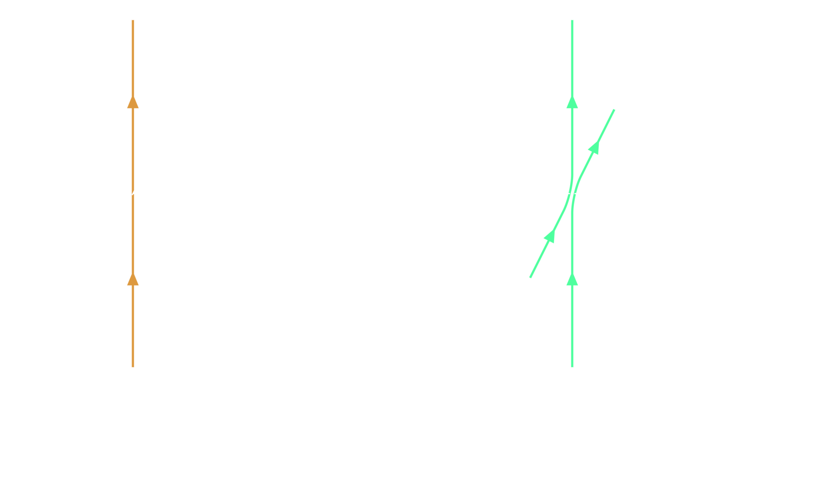
In any case, the resulting non-collisional evolution \(\EvolutionNoninteracting\) from this specification of the time machine is trivial: the particle remains stationary as the past wormhole mouth appears and disappears behind it, while the future mouth later appears and disappears in front of the particle. Nothing passes in or out of the time machine. On the other hand, in the collisional evolution \(\EvolutionInteracting\), a moving particle emerges from the appearing past mouth and strikes the stationary particle, transferring all of its momentum to it. The struck particle then travels into the future mouth that appears directly in front of it, while the other particle becomes stationary and remains so in place of its collision partner. While these trajectories are classical, the particle can be in superpositions of being absent or present on either path. It is stressed that the particle’s position degree of freedom factors out of the evolution because the two classical trajectories coincide in final position and velocity. Therefore, the only relevant degrees of freedom are the internal states of the clock.

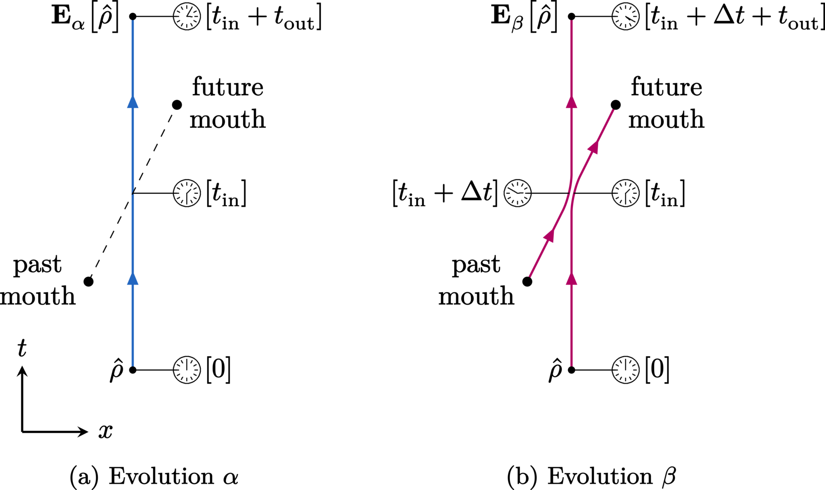
It is also important to note that the incoming past and outgoing future momenta of the billiard-ball clock must exactly match. Assuming a perfectly elastic collision, the combination of the dynamical time machine and the law of conservation of momentum collectively constrains the velocity of the billiard-ball clock on the CTC to a single value (determined by both the geometry of the wormhole and mass of the billiard ball). As a result, there is no need to restrict the paths of the clock (e.g., with waveguides) or its initial velocity because the two distinct, desired histories of our model arise naturally as the only two paths through the spacetime. With this, we can represent the two evolutions of our clock in its reference frame through the chronology-violating region as per Figure 29, where we denote the proper travel time of the clock through the wormhole to be exactly \(\TimeDelta\).

Quantum clocks

For our analysis, we employ the \(\Dimension\)-level, pure, equiprobabilistic quantum clock state

(402)\[\ket{\qclock} = \frac{1}{\sqrt{\Dimension}}\sum_{n=1}^{\Dimension}\ket{n}.\]

Here, the number states \(\{\ket{n}\}_{n=1}^\Dimension\), which obey orthonormality via the condition \(\braket{m}{n} = \delta_{nm}\), collectively form a basis for the \(\Dimension\)-dimensional Hilbert space in which the clock resides. With this, let us define the clock Hamiltonian as

(403)\[\OperatorHamiltonian_\Clock = \sum_{n=1}^{\Dimension} \Energy_n\ket{n}\bra{n}\]

where \(\Energy_n\) is the energy of the \(n\)-th eigenstate \(\ket{n}\). Time evolution of a state over the times \(\TimeInitial\rightarrow\TimeFinal\) is then generated by the time-evolution unitary, which in its standard form may be written

(404)\[\Rotation(\TimeFinal;\TimeInitial) \equiv \Rotation(\TimeFinal-\TimeInitial) = \e^{-\eye\OperatorHamiltonian_\Clock(\TimeFinal-\TimeInitial)/\hbar}.\]

This is written using the standard notation for the rotation operator \(\Rotation\) because the transformation of a clock state produced by “time evolution” is simply a standard rotation operation. Given this form, the evolution of an initial clock state \(\ket{\qclock(\Time)}\) (at time \(\Time\)) to a later state \(\ket{\qclock(\Time+\TimeDelta)}\) (at time \(\Time+\TimeDelta\)) is simply

(405)\[\ket{\qclock(\Time+\TimeDelta)} = \Rotation(\TimeDelta)\ket{\qclock(\Time)} = \e^{-\eye\OperatorHamiltonian_\Clock\TimeDelta/\hbar}\ket{\qclock(\Time)}.\]

Expanding (404) via a Taylor series and subsequently using the Hamiltonian expansion (403) allows us to express an evolved state \(\ket{\qclock(\Time)}\) in terms of its constituent basis states \(\{\ket{n}\}_{n=1}^\Dimension\) as

(406)\[\ket{\qclock(\Time)} = \frac{1}{\sqrt{\Dimension}}\sum_{n=1}^{\Dimension}\e^{-\eye \Energy_n \Time/\hbar}\ket{n}.\]

The overlap between two states at different stages of time evolution is easily calculable as

(407)\[\braket{\qclock(\Time)}{\qclock(\Time+\TimeDelta)} = \frac{1}{\Dimension} \sum_{n=1}^{\Dimension} \e^{-\eye \Energy_n\TimeDelta/\hbar},\]

which quantifies the distinguishability (i.e., coherence) between the two clock states. Now, given our freedom of choice in specifying the energies without losing generality or functionality of the clock, we may choose them to be equally spaced such that

(408)\[\EnergyDelta = \Energy_n - \Energy_{n-1}.\]

Accordingly, the \(n\)-th energy \(\Energy_n\) can be expressed in terms of the ground state \(\Energy_1\) and the spacing \(\EnergyDelta\) as

(409)\[\Energy_n = \Energy_1 + (n-1)\EnergyDelta.\]

From this, we introduce the orthogonalization time of our \(\Dimension\)-level clock, defined as

(410)\[\TimeOrthogonalization = \frac{2\pi\hbar}{\Dimension\EnergyDelta},\]

which represents the minimal time needed for a clock to evolve (under the equally spaced Hamiltonian (403)) into an orthogonal one. A system with finite \(\TimeOrthogonalization\) can be thought of as a clock which “ticks” at a rate proportional to \(\TimeOrthogonalization^{-1}\). Now, using the form (410) and the energy level relation (409) allows us to write the clock overlap (407) as

(411)\[\braket{\qclock(\Time)}{\qclock(\Time+\TimeDelta)} = \frac{\e^{-\eye \Energy_1\TimeDelta/\hbar}}{\Dimension} \sum_{n=1}^{\Dimension} \exp\left[-2\pi\eye\frac{n-1}{\Dimension}\frac{\TimeDelta}{\TimeOrthogonalization}\right].\]

A point to note is that these clocks, when composed of equally spaced energy eigenstates as imposed by (409), are dependent on only two parameters: the time \(\Time\) of their evolution and the energy \(\Energy_1\) of their ground state \(\ket{1}\). Mathematically, this can be shown by using (409) and (410) to express (406) as

(412)\[\ket{\qclock(\Time)} = \frac{\e^{-\eye \Energy_1 \Time/\hbar}}{\sqrt{\Dimension}}\sum_{n=1}^{\Dimension}\exp\left[-2\pi\eye\frac{n-1}{\Dimension}\frac{\Time}{\TimeOrthogonalization}\right]\ket{n}.\]

In any case, by the series identity

(413)\[\sum_{n=1}^{\Dimension} r^{n-1} = \frac{1-r^\Dimension}{1-r}, \qquad r\neq 1,\]

we may write (411) as

(414)\[\braket{\qclock(\Time)}{\qclock(\Time+\TimeDelta)} = \frac{\e^{-\eye \Energy_1\TimeDelta/\hbar}}{\Dimension} \frac{1 - \exp\left[-2\pi\eye\frac{\TimeDelta}{\TimeOrthogonalization}\right]}{1 - \exp\left[-2\pi\eye\frac{1}{\Dimension}\frac{\TimeDelta}{\TimeOrthogonalization}\right]}.\]

Evidently, in the case that the evolution time difference is equal to the orthogonalization time, i.e., \(\TimeDelta = \TimeOrthogonalization\), then from (414) it is easy to see that the clock overlap vanishes, i.e.

(415)\[\left.\braket{\qclock(\Time)}{\qclock(\Time+\TimeDelta)}\right|_{\TimeDelta = \TimeOrthogonalization} = 0.\]

The case of \(\TimeDelta = \TimeOrthogonalization\) can thus be interpreted as when the clock’s “resolution” exactly matches the time difference between the relevant states. This is the key mechanism with which one can investigate temporal differences between the multiple trajectories (such as the two paths in the simple billiard-ball paradox) that are generated via the indeterminism present in spacetimes containing CTCs. Note that such modelling of an internal clock to track a quantum particle’s proper time was first described in [6].

As a final point, note that the simple form of the clock state and its associated Hamiltonian are only convenient choices—the results we obtain from the model of the billiard-ball paradox are completely independent of them (provided the initial clock is not an energy eigenstate but is a superposition of different energies). In particular, given that any quantum system can be decomposed into an orthogonal energy basis, then the use of such a basis poses no restrictions on any findings. The use of uniform \(1/\sqrt{\Dimension}\) weights in the initial state also merely provides simplicity compared to that of general amplitudes \(\{c_n\}_{n=1}^{\Dimension}\). In the same vein, the fact that the energy levels are chosen to be equally spaced means that the orthogonalization time is the same between orthogonal states. Non-equally spaced energies on the other hand would only prevent the simplification of the D-CTC solutions. Indeed, the only consequential assumption which we make of the clock system is that it is finite-dimensional, a fact that can be justified by assuming that the clock states must belong to some set of bound states.

Quantum circuit model of the billiard-ball paradox

We now turn our attention to constructing the quantum circuit model of the simplified billiard-ball paradox. For simplicity, we choose the initial (unevolved) clock state,

(416)\[\StateCR = \ket{\qclock(0)}\bra{\qclock(0)},\]

to be the CR input along the trajectories illustrated in Figure 29. Given these trajectories, it is easy to construct quantum circuit formulations for the clock states, and such circuits appear in Figure 30.

Figure 30 Quantum circuit models of the two trajectories of Figure 29 under study.

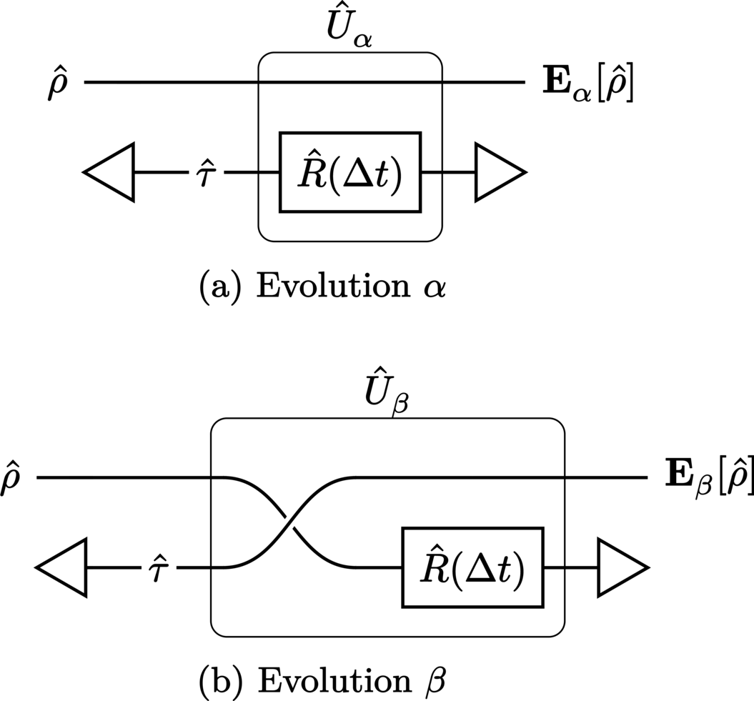
Here, the elastic self-collision of the clock between its past and future selves may be represented by the SWAP gate,

(417)\[\Swap = \sum_{j,k=1}^{\Dimension}{\ket{j}\bra{k}}_\CR\otimes{\ket{k}\bra{j}}_\CV.\]

In effect, this exchange of the CV (trapped CTC) and CR (incoming system) quantum states mimics the momentum-exchange collision interaction between the billiard ball’s past and future selves [which necessarily occurs in \((1+1)\) dimensions]. (Note that here, the basis states correspond to those from which the particle’s wave function is constructed. This means that, in the case of a quantum clock, these basis states represent the number states of the clock’s Hilbert space.) This is because the complete transference of momentum between two particles (here, the past and future versions of the billiard ball) is necessarily an exchange of quantum clock state, provided the associated particles are otherwise identical. To clarify, in a particle’s quantum description, the clock degree of freedom is the identifying attribute, while momentum performs the same function in its classical description. As such, the two necessarily correspond such that when a pair of classically indistinguishable particles trade momentum, they exchange their clocks, i.e., \(\Swap \ket{\qclock(\Time_1)} \otimes \ket{\qclock(\Time_2)} = \ket{\qclock(\Time_2)} \otimes \ket{\qclock(\Time_1)}\).

Additionally, for simplicity, the rotations of the clock on the path sections outside of the CTC (on the CV system between the time machine) have been neglected. This is valid because these time evolutions (namely the inbound \(\TimeInbound\) and outbound \(\TimeOutbound\) times) are experienced by both paths, and so contribute the same to the clock’s total time evolution. This means that a clock which does not interact with the CTC will not evolve, while one which does interact will evolve (by the CTC “duration” \(\TimeDelta\)).

Next, in order to combine the two separate subcircuits of Figure 30 into a single circuit, we introduce a “vacuum” state \(\ket{0}\) (orthonormal to the existing number states) into both the CR and CV Hilbert spaces. Of the many consequences of doing so, perhaps the most significant is that, because the clock’s subspace has \(\Dimension\) dimensions, the total space now has \(\Dimension + 1\) dimensions.

In order to model the paradox faithfully, we mandate that the vacuum and clock cannot “collide” with each other. This effect will be enforced by modifying the SWAP gate to the form

(418)\[\VacuumSwap = \VacuumIdentity_\CR\otimes\ket{0}\bra{0}_\CV + \ket{0}\bra{0}_\CR\otimes\VacuumIdentity_\CV - \ket{0}\bra{0}_\CR\otimes\ket{0}\bra{0}_\CV + \Swap\]

where \(\VacuumIdentity = \Identity + \ket{0}\bra{0}\) is the identity matrix in a vacuum-inclusive Hilbert space. This altered SWAP simply excludes the vacuum from swapping with the non-vacuous states, e.g.,

(419)\[\begin{split}\begin{aligned} \VacuumSwap \ket{0} \otimes \ket{0} &= \ket{0} \otimes \ket{0}, \\ \VacuumSwap \ket{\qclock} \otimes \ket{0} &= \ket{\qclock} \otimes \ket{0}, \\ \VacuumSwap \ket{0} \otimes \ket{\qclock} &= \ket{0} \otimes \ket{\qclock}, \\ \VacuumSwap \ket{\qclock(\Time_1)} \otimes \ket{\qclock(\Time_2)} &= \ket{\qclock(\Time_2)} \otimes \ket{\qclock(\Time_1)}. \end{aligned}\end{split}\]

In this interpretation, the state \(\ket{0}\) represents the physical absence of a clock \(\ket{\qclock}\), hence the “vacuum” nomenclature.

In the associated extended Hilbert space, we write the vacuum-inclusive time-evolution operator as

(420)\[\VacuumRotation(\TimeFinal - \TimeInitial) = \ket{0}\bra{0} + \Rotation(\TimeFinal - \TimeInitial).\]

This form describes the special case where, without loss of generality in the model’s results, the vacuum has vanishing energy such that its time-evolution phase coefficient is unity, i.e.,

(421)\[\bra{0}\VacuumRotation\ket{0} = 1.\]

With this in mind, the corresponding vacuum-modified unitary operator is

(422)\[\UnitaryVacuum = \bigl[\VacuumIdentity_\CR\otimes\VacuumRotation_\CV(\TimeDelta)\bigr]\VacuumSwap.\]

Under this, the input state may either self-consistently interact with the CTC, or it may pass straight through the circuit, thus allowing it to evolve through the circuit in the two paths of Figure 29.

Figure 31 A quantum model of the (simplified) billiard-ball paradox. Here, the SWAP gate is a modified \(\ket{0}\)-excluding variant as defined in (418).

Solutions

The D-CTC solutions can be calculated to be

(423)\[\begin{split}\begin{aligned} \StateCR_{\MapDCTCsCR} &= \ParameterFree\ket{\qclock(0)}\bra{\qclock(0)} + (1 - \ParameterFree)\ket{\qclock(\TimeDelta)}\bra{\qclock(\TimeDelta)}\\ \StateCV_{\MapDCTCsCR} &= \ParameterFree\ket{0}\bra{0} + (1 - \ParameterFree)\ket{\qclock(\TimeDelta)}\bra{\qclock(\TimeDelta)}. \end{aligned}\end{split}\]

Here, \(0 \leq \ParameterFree \leq 1\) is the multiplicity parameter that assumes a value of \(\ParameterFree = \frac{1}{\Dimension + 1}\) in the case of Deutsch’s rule of maximal entropy.

For P-CTCs on the other hand, we first compute the P-CTC operator,

(424)\[\begin{split}\begin{aligned} \OperatorPCTC &\equiv \trace_\CV[\Unitary] \\ &= \trace\bigl[\VacuumRotation(\TimeDelta)\bigr] \ket{0}\bra{0} + \Identity + \Rotation(\TimeDelta). \end{aligned}\end{split}\]

with which the corresponding solution can be determined to be

(425)\[\ket{\StatePure_{\MapPCTCsCR}} = \frac{1}{\sqrt{\Normalization}} \bigl[\ket{\qclock(0)} + \ket{\qclock(\TimeDelta)}\bigr],\]

where

(426)\[\begin{split}\begin{aligned} \Normalization &= \trace[\OperatorPCTC \StateCR \OperatorPCTC^\dagger],\\ &= 2 + \frac{1}{\Dimension}\Bigl(\trace\bigl[\Rotation(\TimeDelta)\bigr] + \trace\bigl[\Rotation^\dagger(\TimeDelta)\bigr]\Bigr). \end{aligned}\end{split}\]

is the normalization factor. Additionally, although it has not been proven to be valid for non-qubit systems, the generalized weak-measurement tomography expression of the P-CTC CV state yields

(427)\[\StateCV_{\MapPCTCsCR} = \frac{1}{\Dimension + 1}\bigl[\ket{0}\bra{0} + \Dimension \ket{\qclock(0)}\bra{\qclock(0)}\bigr].\]

Note how this is exactly the maximally entropic version of the D-CTC solution, as predicted by the theory.

Qubit clocks

A particularly eludicating special case of the model discussed so far is one in which the clock’s subspace is an ordinary qubit space with basis vectors \(\{\ket{1},\ket{2}\}\). Accordingly, an initial (unevolved) clock state appears as

(428)\[\ket{\qclock(0)} = \frac{1}{\sqrt{2}}\bigl(\ket{1} + \ket{2}\bigr).\]

By (409) and (410), the associated clock gate may be written as

(429)\[\Rotation(\TimeDelta) = \e^{-\eye \Energy_1\Delta\Time/\hbar}\bigl(\ket{1}\bra{1} + \e^{-\eye \pi \TimeDelta/\TimeOrthogonalization}\ket{2}\bra{2}\bigr),\]

so that the orthogonalization time \(\TimeDelta = \TimeOrthogonalization\) transforms the initial clock qubit (428) into the orthogonal state

(430)\[\ket{\qclock(\TimeOrthogonalization)} = \Rotation(\TimeOrthogonalization)\ket{\qclock(0)} = \frac{\e^{-\eye \Energy_1\TimeOrthogonalization/\hbar}}{\sqrt{2}}\bigl(\ket{1}-\ket{2}\bigr).\]

Importantly, note that qubit clocks only have two mutually orthogonal states, which means that multiple loops of the CTC cannot be distinguished by such clocks.

In this \(3\)-dimensional total Hilbert space (of both the vacuum and the clock), we compute the D-CTC solutions to be

(431)\[\begin{split}\begin{aligned} \StateCR_{\MapDCTCsCR} &= \frac{1}{2}\Bigl[\ket{1}\bra{1} + \bigl(\ParameterFree + (1 - \ParameterFree)\e^{\eye \pi \TimeDelta/\TimeOrthogonalization}\bigr)\ket{1}\bra{2} + \bigl(\ParameterFree + (1 - \ParameterFree)\e^{-\eye \pi \TimeDelta/\TimeOrthogonalization}\bigr)\ket{2}\bra{1} + \ket{2}\bra{2}\Bigr]\\ \StateCV_{\MapDCTCsCR} &= \ParameterFree\ket{0}\bra{0} + (1 - \ParameterFree)\frac{1}{2}\Bigl[\ket{1}\bra{1} + \e^{\eye \pi \TimeDelta/\TimeOrthogonalization}\ket{1}\bra{2} + \e^{-\eye \pi \TimeDelta/\TimeOrthogonalization}\ket{2}\bra{1} + \ket{2}\bra{2}\Bigr], \end{aligned}\end{split}\]

while the P-CTC solutions are

(432)\[\begin{split}\begin{aligned} \ket{\StatePure_{\MapPCTCsCR}} &= \frac{1}{\sqrt{3 + \cos\left(\frac{\TimeDelta}{\TimeOrthogonalization}\pi\right)}} \bigl[\ket{\qclock(0)} + \ket{\qclock(\TimeDelta)}\bigr] \\ &\propto 2\ket{1} + (1 + \e^{-\eye \pi \TimeDelta/\TimeOrthogonalization})\ket{2}, \\ \StateCV_{\MapPCTCsCR} &= \frac{1}{3}\bigl[\ket{0}\bra{0} + 2 \ket{\qclock(0)}\bra{\qclock(0)}\bigr]. \end{aligned}\end{split}\]

P-CTC restrictions on initial data

One interesting general characteristic of P-CTCs is that they can pose constraints on initial conditions. Due to the renormalization, such constraints depend on the future of the time-travelling state. Here, we explicitly demonstrate the restrictions associated with the P-CTCs description of the circuit.

Given the \(\Dimension\)-level clock (402), there exist exactly \(\Dimension\) mutually orthogonal, equally spaced states \(\bigl\{\ket{\qclock^{(k)}(\TimeOrthogonalization)}\bigr\}_{k=0}^{\Dimension-1}\) of which it can assume. As a consequence, one may express the clock gate (404) in terms of the ground-state energy \(\Energy_1\) (defined via (409)) as

(433)\[\Rotation(\TimeFinal - \TimeInitial) = \e^{-\eye \Energy_1 (\TimeFinal - \TimeInitial)/\hbar} \sum_{n=1}^{\Dimension}\exp\left[-2\pi\eye\frac{n-1}{\Dimension}\frac{\TimeFinal - \TimeInitial}{\TimeOrthogonalization}\right]\ket{n}\bra{n}.\]

From this, it is easy to conclude that

(434)\[\Rotation^\Dimension(\TimeOrthogonalization) = \e^{-\eye \Dimension \Energy_1 \TimeOrthogonalization/\hbar}\Identity,\]

which simply indicates that \(\Dimension\) orthogonal rotations of the clock return it to its initial state, up to the global phase \(\e^{-\eye \Dimension \Energy_1 \TimeOrthogonalization/\hbar}\). Accordingly, a clock \(\ket{\qclock}\) that orthogonalizes \(p\in\Integers_{>0}\) times accumulates \(p\) such phases. Therefore, judicious choice of the clock’s orthogonalization time \(\TimeOrthogonalization\), such that it is related to the CTC time delay \(\TimeDelta\) by

(435)\[\TimeDelta = p \Dimension \TimeOrthogonalization,\]

means that a clock which completes one journey on the CTC would orthogonally evolve \(p\) times. In such a case, the P-CTC reduced operator (424) becomes

(436)\[\left.\OperatorPCTC\right|_{\TimeDelta = p \Dimension \TimeOrthogonalization} = \left(1 + \Dimension \e^{-\eye p \Dimension \Energy_1 \TimeOrthogonalization/\hbar}\right)\ket{0}\bra{0} + \left(1 + \e^{-\eye p \Dimension \Energy_1 \TimeOrthogonalization/\hbar}\right)\Identity.\]

Additionally, if we construct the clock so that its ground-state energy \(\Energy_1\) satisfies

(437)\[\Energy_1 = \frac{\pi\hbar}{p \Dimension \TimeOrthogonalization}(1 + 2q),\quad q\in\Integers_{\geq 0},\]

then the operator (436) further reduces to

(438)\[\begin{split}\OperatorPCTC' = \left.\OperatorPCTC\right|_{\substack{\TimeDelta = p \Dimension \TimeOrthogonalization\\ \Energy_1 = \frac{\pi\hbar}{p \Dimension \TimeOrthogonalization}(1 + 2q)}} = \left(1 - \Dimension\right)\ket{0}\bra{0}.\end{split}\]

After renormalization, the corresponding P-CTC output is then, of course, simply the vacuum state, i.e., \(\ket{0}\). This cannot be valid however, because the initial input state (416) did not include any vacuum term. So what happened to the clock?

To answer this question, we can use the vacuum-including entangled state

(439)\[\ket{\StatePure}_{\text{rec},\CR} = \sqrt{\ParameterVacuum}\ket{0}_\text{rec}\otimes\ket{0}_\CR + \sqrt{1 - \ParameterVacuum}\ket{\qclock(0)}_\text{rec}\otimes\ket{\qclock(0)}_\CR, \quad 0 \leq \ParameterVacuum \leq 1,\]

as input to our circuit. Here, the state existing in the first system may be interpreted as a record of what we send into the CR system. With this entanglement, we find the P-CTC unnormalized pure-state output, corresponding to our circuit’s ordinary operator \(\VacuumIdentity_\text{rec}\otimes\OperatorPCTC_\CR\) from (424), to be

(440)\[\begin{split}\begin{aligned} \bigl(\VacuumIdentity_\text{rec}\otimes\OperatorPCTC_\CR\bigr)\ket{\StatePure}_{\text{rec},\CR} &\propto \sqrt{\ParameterVacuum}\,\trace[\VacuumRotation(\TimeDelta)]\,\ket{0}_\text{rec}\otimes\ket{0}_\CR \\ &\quad + \sqrt{1 - \ParameterVacuum}\,\ket{\qclock(0)}_\text{rec}\otimes\bigl[\ket{\qclock(0)}_\CR + \ket{\qclock(\TimeDelta)}_\CR\bigr]. \end{aligned}\end{split}\]

The persistence of the entanglement means that when the record indicates that we did not send in a clock, we will not observe a clock in the CR output. Conversely, when we definitely did send in a clock, we must observe a clock exiting the CTC region, which is exactly what one intuitively expects. However, under the conditions (435) and (437) which yield the operator (438), the entanglement of our input state (439) breaks,

(441)\[\bigl(\VacuumIdentity_\text{rec}\otimes\OperatorPCTC'_\CR\bigr)\ket{\StatePure}_{\text{rec},\CR} \propto \ket{0}_\text{rec}\otimes\ket{0}_\CR,\]

regardless of the value of \(\ParameterVacuum\) (provided it is non-zero). Thus, the mere presence of the interaction with the CTC in the future implies that the record subsystem will show that no clock was ever prepared, even though the initial state (439) included the possibility that a clock was there (which would show up in the record if the future interaction with the CTC was avoided).

Given the path-integral correspondence of P-CTCs, the conditions (435) and (437) collectively form a case in which no clocks can evolve through the circuit due to destructive interference in the path integral. This is to say that P-CTCs suppress all evolutions of non-vacuous states as a result of the particular future evolution of clock states in our model, thereby posing constraints on the initial state. This issue highlights the well-known problem of antichronological and superluminal influence with P-CTCs [2, 3, 9]. In contrast, the initial data for D-CTCs are never affected by the presence (or absence) of a CTC in the future.

Implementation

This implementation is strictly for qubits. For simplicity, we set \(\frac{\TimeDelta}{\TimeOrthogonalization} \equiv t\).

Listing 29 /text/examples/ctcs/billiards.py

from qhronology.quantum.states import VectorState
from qhronology.quantum.gates import QuantumGate, Swap, Diagonal
from qhronology.quantum.prescriptions import QuantumCTC, DCTC, PCTC

import sympy as sp
from sympy.physics.quantum import TensorProduct

# Input
clock_state_unevolved = VectorState(spec=[[0, 1, 1]], dim=3, norm=1, label="ψ")
clock_state_evolved = VectorState(spec=[[0, 1, -1]], dim=3, norm=1, label="ψ")

# Gates
I = QuantumGate(
    spec=[[1, 0, 0], [0, 1, 0], [0, 0, 1]], targets=[0], num_systems=1, dim=3
)
zero = QuantumGate(
    spec=[[1, 0, 0], [0, 0, 0], [0, 0, 0]], targets=[0], num_systems=1, dim=3
)
S = Swap(targets=[0, 1], num_systems=2, dim=3)
IR = Diagonal(
    entries={2: "-pi*t"},
    exponentiation=True,
    symbols={"t": {"real": True, "positive": True}},
    targets=[1],
    num_systems=2,
    dim=3,
    label="R",
)

# Construct SWAP gate in clock subspace
S = sp.Matrix(9, 9, lambda i, j: 0 if i % 3 == 0 or j % 3 == 0 else S.matrix[i, j])

# Construct vacuum-excluding SWAP gate
S_vacuum = QuantumGate(
    spec=(
        TensorProduct(I.matrix, zero.matrix)
        + TensorProduct(zero.matrix, I.matrix)
        - TensorProduct(zero.matrix, zero.matrix)
        + S
    ),
    targets=[0, 1],
    num_systems=2,
    dim=3,
    family="SWAP",
)

# CTC
billiards = QuantumCTC(
    inputs=[clock_state_unevolved], gates=[S_vacuum, IR], systems_respecting=[0]
)
billiards.diagram()

# Output
# D-CTCs
billiards_DCTC = DCTC(circuit=billiards)
billiards_DCTC_respecting = billiards_DCTC.state_respecting(norm=False, label="ρ_D")
billiards_DCTC_violating = billiards_DCTC.state_violating(norm=False, label="τ_D")
billiards_DCTC_respecting.simplify()
billiards_DCTC_respecting.apply(sp.factor)

# P-CTCs
billiards_PCTC = PCTC(circuit=billiards)
billiards_PCTC_respecting = billiards_PCTC.state_respecting(norm=False, label="ψ_P")
billiards_PCTC_violating = billiards_PCTC.state_violating(norm=False, label="τ_P")
billiards_PCTC_respecting.normalize(1)

# Results
billiards_DCTC_respecting.print()
billiards_DCTC_violating.print()
billiards_PCTC_respecting.print()
billiards_PCTC_violating.print()

Output

Diagram

>>> billiards.diagram()

States

>>> billiards_DCTC_respecting.print()
ρ_D = 1/2|1⟩⟨1| + -(g*exp(I*pi*t) - g - exp(I*pi*t))/2|1⟩⟨2| + (g*exp(I*pi*t) - g + 1)*exp(-I*pi*t)/2|2⟩⟨1| + 1/2|2⟩⟨2|

>>> billiards_DCTC_violating.print()
τ_D = g|0⟩⟨0| + (1/2 - g/2)|1⟩⟨1| + (1 - g)*exp(I*pi*t)/2|1⟩⟨2| + (1 - g)*exp(-I*pi*t)/2|2⟩⟨1| + (1/2 - g/2)|2⟩⟨2|

>>> billiards_PCTC_respecting.print()
|ψ_P⟩ = sqrt(2)*sqrt(1/(cos(pi*t) + 3))|1⟩ + sqrt(2)*(1 + exp(-I*pi*t))*sqrt(1/(cos(pi*t) + 3))/2|2⟩

>>> billiards_PCTC_violating.print()
τ_P = 1/3|0⟩⟨0| + 1/3|1⟩⟨1| + exp(I*pi*t)/3|1⟩⟨2| + exp(-I*pi*t)/3|2⟩⟨1| + 1/3|2⟩⟨2|

References

[1]

T. C. Ralph and T. G. Downes, “Relativistic quantum information and time machines”, Contemporary Physics, 53(1):1–16, January 2012. http://www.tandfonline.com/doi/abs/10.1080/00107514.2011.640146, doi:10.1080/00107514.2011.640146

[2] (1,2,3)

J. Friedman, M. S. Morris, I. D. Novikov, F. Echeverria, G. Klinkhammer, K. S. Thorne, and U. Yurtsever, “Cauchy problem in spacetimes with closed timelike curves”, Physical Review D, 42(6):1915–1930, September 1990. https://link.aps.org/doi/10.1103/PhysRevD.42.1915, doi:10.1103/PhysRevD.42.1915

[3]

J. Bub and A. Stairs, “Quantum interactions with closed timelike curves and superluminal signaling”, Physical Review A, 89(2):022311, February 2014. https://link.aps.org/doi/10.1103/PhysRevA.89.022311, doi:10.1103/PhysRevA.89.022311

[4]

S. Ghosh, A. Adhikary, and G. Paul, “Quantum signaling to the past using P-CTCS”, Quantum Information and Computation, 18(11&12):965–974, September 2018. http://www.rintonpress.com/journals/doi/QIC18.11-12-5.html, doi:10.26421/QIC18.11-12-5

[5]

L. G. Bishop, F. Costa, and T. C. Ralph, “Time-traveling billiard-ball clocks: A quantum model”, Physical Review A, 103(4):042223, April 2021. https://link.aps.org/doi/10.1103/PhysRevA.103.042223, doi:10.1103/PhysRevA.103.042223

[6]

M. Zych, F. Costa, I. Pikovski, and Č. Brukner, “Quantum interferometric visibility as a witness of general relativistic proper time”, Nature Communications, 2:505, October 2011. http://www.nature.com/articles/ncomms1498, doi:10.1038/ncomms1498